Excel IMAGE function – quick way to insert picture in cell with formula
Discover an incredibly easy way to insert a picture into a cell using the IMAGE function!
For years, Microsoft Excel users had to go through a long and tricky process to add pictures to worksheets. But now, that hassle is gone! With the new IMAGE function, you can insert pictures directly into cells using a simple formula. You can also place images in Excel tables, move, copy, resize, sort, and filter them just like regular cells. Instead of floating on top of the spreadsheet, your images now become a real part of it
Table of Contents
Excel IMAGE function
The IMAGE function in Excel lets you insert pictures directly into cells using a URL. It supports these file formats: BMP, JPG/JPEG, GIF, TIFF, PNG, ICO, and WEBP.
This function has 5 parts, but you only need to use the first one.
Here’s what each part means:
- Source (required): The web link (URL) of the image, using “https”. You can type the link in double quotes or refer to a cell that contains the URL.
- Alt_text (optional): A description of the image.
- Sizing (optional): Controls how the image fits in the cell:
- 0 (default): Fits the image in the cell while keeping its shape.
- 1: Stretches the image to fill the cell, ignoring its shape.
- 2: Keeps the original image size, even if it goes outside the cell.
- 3: Lets you set a custom height and width.
- Height (optional): The image height in pixels.
- Width (optional): The image width in pixels.
With this function, adding images to Excel has never been easier!
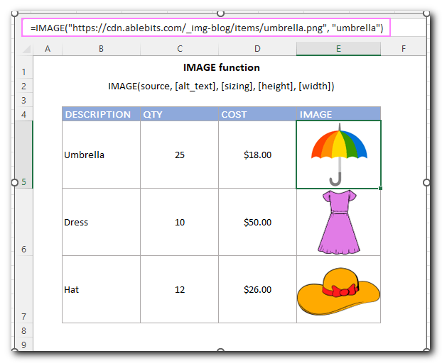
IMAGE function availability
IMAGE is a new function, which is currently available only to Microsoft 365 users for Windows, Mac and Android as well as in Excel for the web.
Basic IMAGE formula in Excel
To create a simple IMAGE formula, you only need to provide the first part—the URL of the image. Just remember:
- The link must use HTTPS (not HTTP).
- Put the URL inside double quotes, just like regular text.
- You can also add a description of the image as the second part.
For example:
=IMAGE(“https://cdn.ablebits.com/_img-blog/image-function/items/umbrella.png”, “umbrella”)
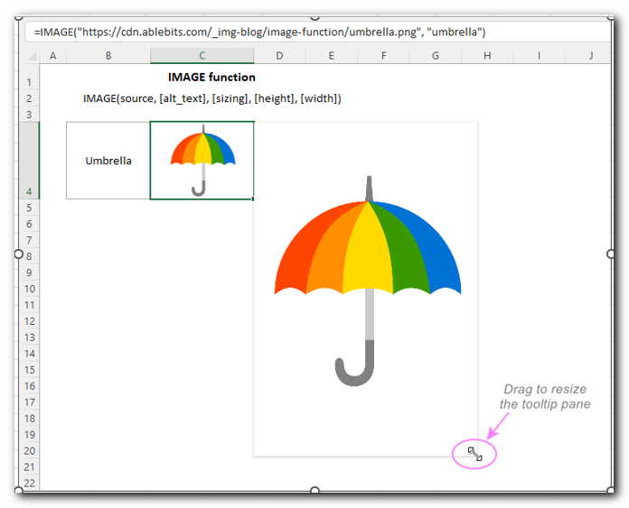
If you skip the third part or set it to 0, the image will automatically fit inside the cell while keeping its original shape. If you resize the cell, the image will adjust too.
When you hover over the cell with an IMAGE formula, a small preview (tooltip) appears. To make this preview bigger, drag its lower-right corner
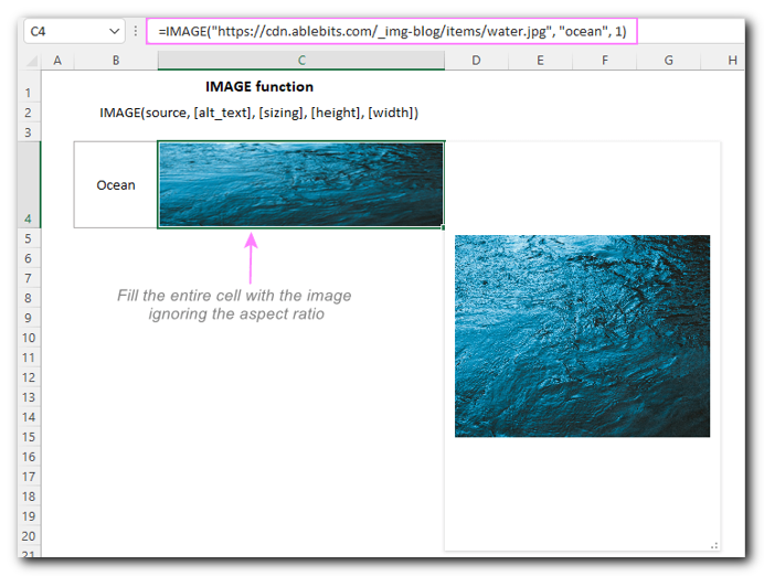
To fill the whole cell with an image, set the 3rd argument to 1. For example:
=IMAGE(“https://cdn.ablebits.com/_img-blog/image-function/items/water.jpg”, “ocean”, 1)
Normally, this works nicely for abstract arts images that look well with almost any width-to-height ratio.
If you want to set a custom height and width for your image (the 4th and 5th parts of the formula), make sure the cell is big enough to fit the full picture. If the cell is too small, only part of the image will show.
Once the image is in the cell, you can copy it easily:
- Just copy the formula to another cell.
- Or, you can reference a cell that already has an IMAGE formula, just like a regular cell.
For example, to copy an image from C4 to D4, simply type
How to insert pictures in Excel cells - formula examples
Introducing the IMAGE function in Excel has “unlocked” many new scenarios that were previously impossible or highly complicated. Below you will find a couple of such examples.
How to make a product list with pictures in Excel
With the IMAGE function, adding product pictures to an Excel list is super easy! Just follow these steps:
- Create or import your product list.
- Make a new list in Excel, import one from a CSV file, or use a product inventory template in Excel.
- Upload your product images online.
- Store them in a folder on your website so each image has a URL.
- Create the IMAGE formula for the first product.
- In the formula, you only need the first part (URL of the image). The second part (alternative text) is optional.
- Copy the formula down the Image column.
- This will quickly apply the same structure to all items.
- Update each IMAGE formula with the correct file name.
- Since all pictures are in the same folder, you just need to change the file name (and alternative text if needed).
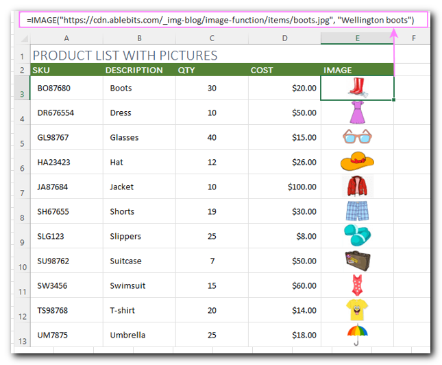
For example, if the product is Wellington boots, enter this in E3:
=IMAGE(“https://cdn.ablebits.com/_img-blog/image-function/items/boots.jpg”, “Wellington boots”)
Now, your product list in Excel will have clear images for easy viewing!
How to return an image based on another cell value
In this example, we will create a drop-down list for selecting items, and when you pick an item, the related picture will appear in the next cell.
Since we want the drop-down list to update automatically when new items are added, we first need to convert the data into an Excel table:
- Select your data and press Ctrl + T to turn it into a table.
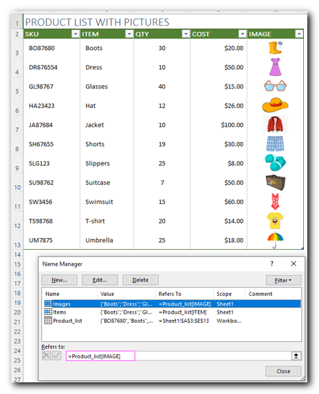
- Once the table is created, give it a name (we named ours Product_list).
Next, we create named ranges for the Item and Image columns (excluding headers):
- Items refers to → =Product_list[ITEM]
- Images refers to → =Product_list[IMAGE]
Now, whenever a new item is selected from the drop-down, the matching image will instantly appear next to it!
to set up the drop-down list, follow these steps:
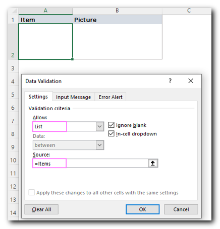
- Click on the cell where you want the drop-down menu.
- Go to the Data tab at the top.
- In the Data Tools group, click Data Validation.
- In the settings, choose List as the validation type.
- For the Source, type =Items (since we named our list Items earlier).
Now, the drop-down will show all the items from your list automatically!
In the cell where you want the image to appear, enter this XLOOKUP formula:
=XLOOKUP(A2, Product_list[ITEM], Product_list[IMAGE])
Here’s how it works:
- A2 → This is the drop-down cell where you select an item.
- Product_list[ITEM] → This tells Excel to search for the selected item in the ITEM column.
- Product_list[IMAGE] → This tells Excel to return the matching image from the IMAGE column.
Since we are looking up values in a table, we use structured references instead of regular cell ranges.
Now, when you pick an item from the drop-down list, the correct image will automatically appear in the next cell!
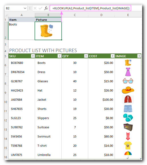
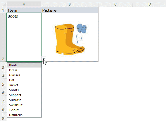
And here’s our dropdown list with related pictures in action – as soon as an item is selected in A2, its image is immediately displayed in B2:
How to make a dropdown with pictures in Excel
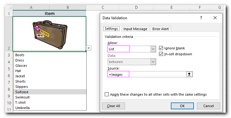
Earlier versions of Excel didn’t allow pictures in a drop-down list. But with the new IMAGE function, this is now possible! You can create a drop-down of pictures in just 4 simple steps:
- Define two names for your dataset:
- Product_list: This is the source table (for example, A10:E20).
- Images: This refers to the IMAGE column in the table, excluding the header.
For more details on how to define names in Excel, check out “How to define a name in Excel.”
- For each IMAGE formula, set the alt_text argument to whatever you want the alternative text to show in the drop-down list.
- In A2, create a drop-down list with the Source set to =Images.
Now, your drop-down will display images alongside their names, making your list more interactive
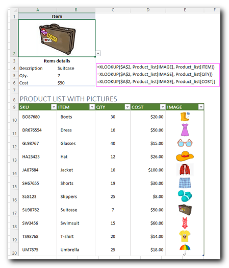
You can also get more details about the selected item using these simple formulas:
- Get the item name:
=XLOOKUP($A$2, Product_list[IMAGE], Product_list[ITEM]) - Get the quantity:
=XLOOKUP($A$2, Product_list[IMAGE], Product_list[QTY]) - Get the cost:
=XLOOKUP($A$2, Product_list[IMAGE], Product_list[COST])
Since the data is stored in a table, the formula uses table and column names instead of regular cell ranges. This makes it easier to manage and update.
Now, when you select an item from the drop-down with images, Excel will automatically show its name, quantity, and cost
Excel IMAGE function known issues and limitations
The IMAGE function is still in beta testing, so it may have a few issues—this is normal! 😊
Here are some things to keep in mind:
- You can only use images from external “https” websites.
- Pictures from OneDrive, SharePoint, or local networks won’t work.
- If a website requires login to view the image, the picture won’t show in Excel.
- Switching between Windows and Mac may cause display problems.
- GIF images are supported, but they appear as static pictures (no animation).
And that’s how you can insert pictures into cells using the IMAGE function!
Thanks for reading, and see you on our blog next week!


