Spill Ranges in Excel: Dynamic Formulas Made Easy
This tutorial breaks down the concept of “spill range” in simple terms and clears up common doubts.
Spilling is a feature in Excel 365 that works with dynamic arrays. Knowing a few key terms will help you get the most out of it.
This makes it easier to follow examples and build your own dynamic array formulas.
The main aim of this tutorial is to help you understand what a spill range is and how it functions.
Table of Contents
Spill range in Excel
When a dynamic array formula returns multiple results, Excel automatically fills the surrounding cells with those extra values.
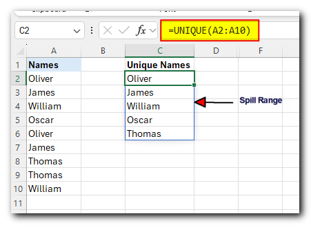
The group of cells that gets filled is called the spill range. It contains all the outputs from the formula.
If you click on any cell within this group, Excel highlights the entire range with a blue border.
This indicates that all values inside the blue box are generated by the formula in the top-left cell.
In the past, with older array formulas (known as CSE formulas), you had to select the right number of cells before entering the formula.
Now, with dynamic arrays, you just enter the formula in one cell, and Excel fills in the rest automatically.
The spill range updates by itself. If your data changes — for example, if you add or remove items — the spill range adjusts to fit.
If you delete the formula from the top cell, all the values in the spill range disappear as well.
Spill range reference (# operator)
To refer to an entire spill range, add a hash symbol (#) after the address of the top-left cell—the one containing the formula that returns multiple values. This is known as a spill range reference in Excel.
For example, if a UNIQUE formula in cell C2 returns several results, you can reference all of them by typing:
To reference the same spill range from a different sheet, include the sheet name followed by an exclamation mark:
To refer to a spill range from another workbook, include the workbook name in square brackets:

Using C2# in a formula works just like using a regular range (such as C2:C5).
But the # symbol is smarter — it automatically expands or shrinks as your data changes, so you don’t need to update your formulas manually.
This is especially useful when you use the spill range inside another function (whether dynamic or standard).
You can even use spill range references in named ranges or data validation lists — like a dropdown that updates itself as new data is added.
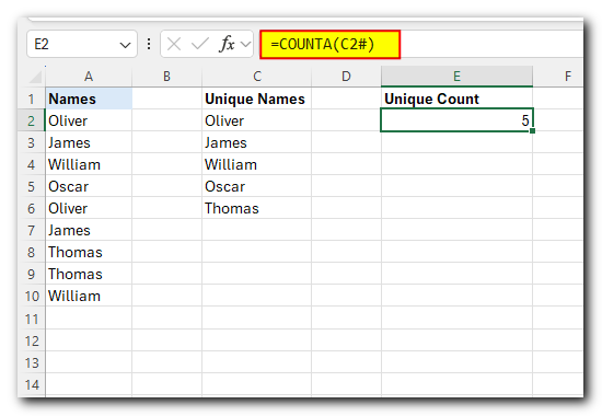
For example, to count how many unique names are returned by the dynamic array in C2, you’d use:
No matter how your list changes, this formula always counts the right number of names.
3 things you should know about Excel spill range
The spill range is a helpful feature in Excel that makes working with dynamic formulas easier and more efficient. Here are three important things to know about how it works:
1. Only the Top-Left Cell Can Be Edited
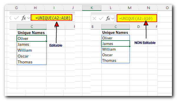
The formula exists only in the top-left cell of the spill range — that’s the only cell you can edit.
If you click on any other cell within the blue-bordered area, the formula will appear in the formula bar but will be greyed out, meaning it can’t be changed from there.
When you edit the top cell and press Enter, Excel automatically refreshes all the results in the spill range.
2. The Spill Range Adjusts Automatically
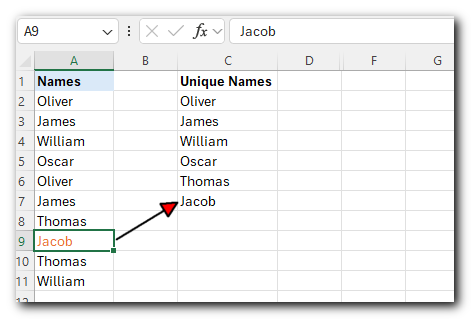
The spill range is dynamic — it grows or shrinks based on the data it returns.
For instance, if your formula pulls in a list of unique names and a new name (like “Jacob”) appears, the spill range will expand to include it automatically.
3. Use Tables or Dynamic Ranges for Best Results
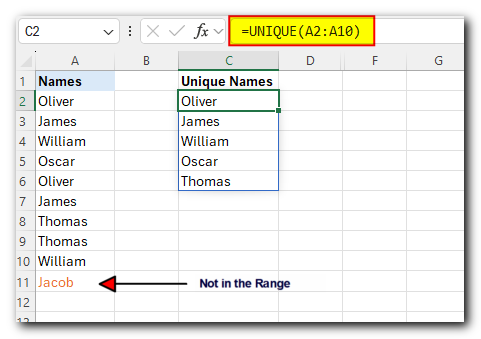
If your source data changes frequently, it’s smart to use an Excel Table or a dynamic named range.
For example, instead of using a fixed range like A2:A10, convert your list into a table. Then use structured references in your formula.
Tables expand automatically when new data is added, so your formula stays up to date without manual edits.
Dynamic named ranges offer another way to ensure your formulas include new data automatically.
#SPILL error
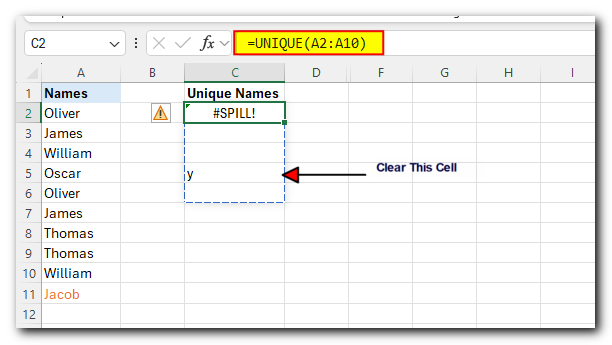
If something is blocking the spill range — such as other data, hidden characters, blank spaces, or existing formulas — Excel will show a #SPILL! error.
To fix it, simply clear the cells that are in the way of the spill range. Once the space is free, Excel will fill in the values as expected.
For more details, check out: SPILL error in Excel – causes and fixes.
To wrap things up, here are answers to three frequently asked questions (3 really is the magic number in this tutorial 
How do you clear a spill range in Excel?
Depending on what you need, here are two simple solutions:
- If you see a #SPILL! error because the spill area isn’t empty, you can:
- Clear the cells that are blocking the spill range, or
- Move the formula to a different location with enough empty space for all the results.
(For more details, check the link above.)
- If you want to remove all the values in the spill range, just delete the formula in the top-left cell — Excel will clear the entire spill area automatically.
How do you change spill range in Excel?
Because the spill range is the output of a formula, you can’t change it manually by selecting cells.
If you want to modify or update the spill range, edit the formula in the top-left cell of the spill area.
Make your changes there and press Enter — Excel will recalculate and adjust the spill range automatically.
How do you fix a spill range if it's too big?
The size of a spill range is determined by Excel and adjusts automatically whenever your source data or formula changes.
In certain cases, you can control the spill range size directly within the formula. For example, you can limit the number of rows returned by functions like FILTER. (Check out: How to limit the number of rows returned by FILTER.)
If you ever encounter a #SPILL! error, this guide can help: How to fix a #SPILL! error in Excel.
How do you get rid of spill range in Excel?
It depends on what you want to do:
- Turn off spilling completely:
You can’t turn off the spill feature for all of Excel. There’s no setting for that because spilling is a helpful tool. It’s better to learn how to use it effectively. - Remove a spill range:
To delete the spill range, just delete the formula in the first (top-left) cell. All the spilled values will disappear. - Stop a formula from spilling into many cells:
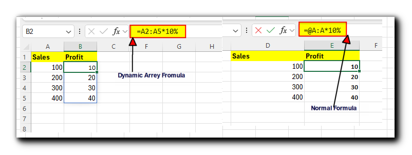
You can use the @ symbol to make the formula return only one value. This is called implicit intersection.
For example, if you write:
Excel multiplies each value in A2 to A5 by 10% and shows the results in four cells.
But if you only want to calculate one value (from the same row), you can use:
This way, only one value is returned.
Now, you are no longer a novice as far as Excel spill range is concerned, right? I thank you for reading and hope to see you on our next blog!
Download Practice File
You can also practice this through our practice files. Click on the below link to download the practice file.


