Excel TEXTAFTER function: retrieves text that appears after a specified character or word.
When dealing with large or complex datasets in Excel, you may need to extract information that follows a specific word or symbol. In this tutorial, you’ll learn a quick and easy method to do that using the new TEXTAFTER function.
Table of Contents
TEXTAFTER function in Excel
The Excel TEXTAFTER function returns the portion of text that comes after a specified character or word, known as the delimiter. If the delimiter appears multiple times, you can select which occurrence to extract text after.
If the delimiter isn’t found, the function can display an error (#N/A), a custom message you define, or simply return the original text.
The syntax for the TEXTAFTER function looks like this:
TEXTAFTER(text, delimiter, [instance_num], [match_mode], [match_end], [if_not_found])
This function has 6 arguments, but only the first two are required:
- text (required):
The original text you want to extract from. It can be a hardcoded string (like “apple”) or a reference to a cell (like A1). - delimiter (required):
The character or word that marks where Excel should start extracting text from. - instance_num (optional):
Tells Excel which occurrence of the delimiter to use.
- Default is 1 (first occurrence).
- Use a negative number to count from the end of the text (e.g., -1 for the last occurrence).
- match_mode (optional):
Controls case sensitivity when looking for the delimiter.
- 0 (default): Case-sensitive
- 1: Case-insensitive
- match_end (optional):
Decides whether the end of the text should act as a delimiter.
- 0 (default): Only matches the exact delimiter
- 1: Treats the end of the text as a delimiter
- If the delimiter isn’t found and instance_num is 1 → returns an empty string
- If instance_num is -1 → returns the entire text
- if_not_found (optional):
What Excel should show if the delimiter isn’t found.
- If left blank, Excel returns #N/A
- You can customize this to show a message (like “Not found”) or return the original text.
Basic Excel text after formula
Let’s start with the basics and learn how to create a simple TEXTAFTER formula in Excel using just the two main parts it needs
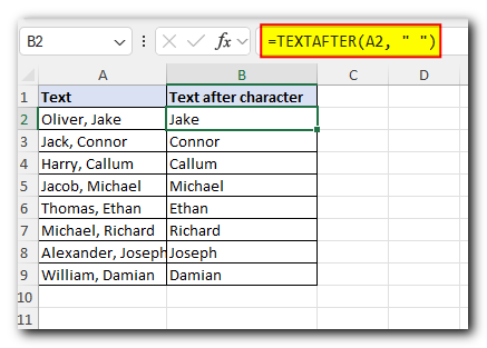
Excel formula: extract text after character
To get the text that comes after a certain character, you first give the cell that has the original text, then put the character (in quotes) that you want to search for. For example, to get the text after a space, the formula looks like this
=TEXTAFTER(A2, ” “)
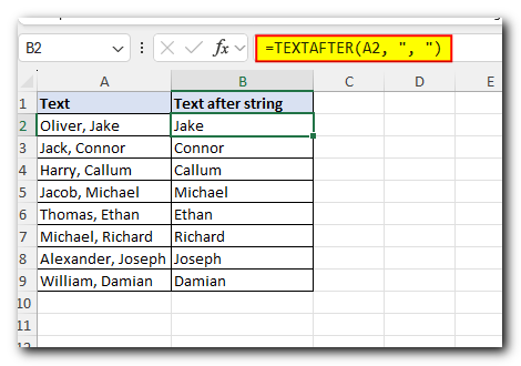
Excel formula: get text after string
If you want to get the text that comes after a specific word or part of a word, use that part as the delimiter. For example, if a comma and space separate last names and first names, use “, ” as the delimiter like this
=TEXTAFTER(A2, “, “)
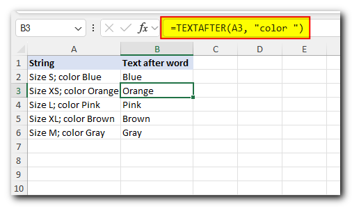
Excel formula: extract text after word
In Excel, a ‘word’ is just a small part of the text, also called a ‘substring’. So, if you want to copy everything that comes after a certain word, use that word as the delimiter.
Example:
To get the text after the word ‘color’, use this formula:
=TEXTAFTER(A2, “color “)
Tip: Don’t forget to include a space after the word ‘color’ in the formula. This helps remove any extra spaces at the beginning of the result.”
Now that you’ve got a grasp of the basics, let’s investigate a few more complex scenarios.
Return text after Nth occurrence of delimiter
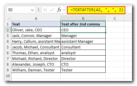
If you want to get the text that comes after the second, third, or any specific time a character appears, you can use the instance_num part of the formula.
For example, to get the text after the second comma, use “, ” as the separator and 2 as the instance number:
=TEXTAFTER(A2, “, “, 2)
Note: The space after the comma is important because the items in the text are separated by a comma and a space
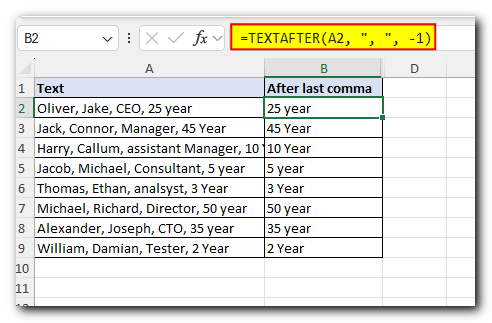
Get text after last occurrence of delimiter
If you want to get the text that comes after the last time a character appears, use a negative number for the instance number.
For example, to get the text after the last comma in cell A2, use -1 like this:
=TEXTAFTER(A2, “, “, -1)
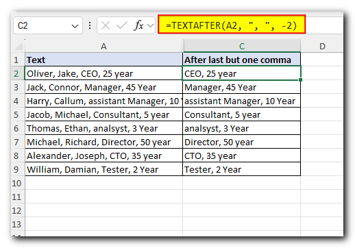
To extract the text after the last but one comma, set instance_num to -2:
=TEXTAFTER(A2, “, “, -2)
Get text after multiple delimiters
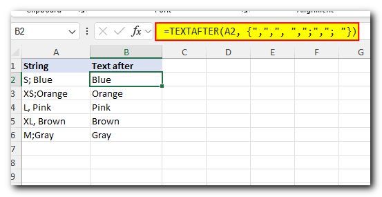
If your text uses different characters to separate parts—like commas or semicolons—you can tell Excel to look for all of them at once using a list called an ‘array constant’, like this: {“x”, “y”, “z”}.
For example, if your text has commas and semicolons, sometimes with spaces, you can use this list: {“,”, “, “, “;”, “; “}
Here’s the formula:
=TEXTAFTER(A2, {“,”, “, “, “;”, “; “})
This will work with any of those separators and pull out the text that comes after them.
If delimiter not found, return your own text
If your text uses different characters to separate parts—like commas or semicolons—you can tell Excel to look for all of them at once using a list called an ‘array constant’, like this: {“x”, “y”, “z”}.
For example, if your text has commas and semicolons, sometimes with spaces, you can use this list: {“,”, “, “, “;”, “; “}
Here’s the formula:
=TEXTAFTER(A2, {“,”, “, “, “;”, “; “})
This will work with any of those separators and pull out the text that comes after them.
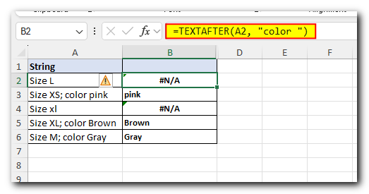
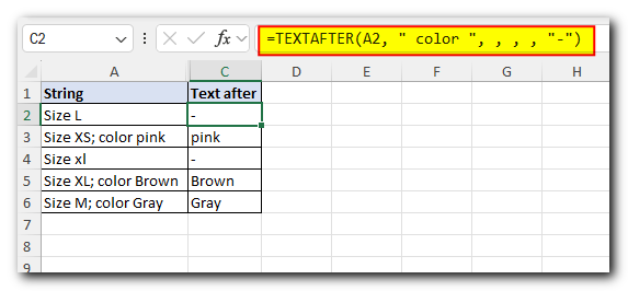
To return a blank cell instead, we supply an empty string (“”) for if_not_found:
=TEXTAFTER(A2, “color “, , , , “”)
Alternatively, you can type any text or character you want, say a hyphen “-“:
=TEXTAFTER(A2, “color “, , , , “-“)
If delimiter is not found, return original text
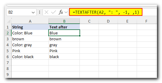
If you want to return the full original text when TEXTAFTER can’t find the word or symbol you’re looking for, here’s how to do it:
- Set instance_num to -1 so Excel searches from right to left.
- Set match_end to 1 so Excel treats the end of the text as the fallback point.
This way, if the delimiter isn’t found, Excel gives you the whole text instead of an error.
For example, if you’re looking for a colon and space (“: “), use this formula:
=TEXTAFTER(A2, “: “, -1, , 1)
If there’s no colon and space in the text, the entire content of the cell will be shown.
TEXTAFTER formula case-sensitive and case-insensitive
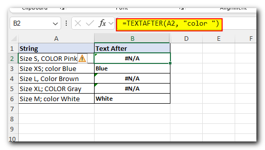
By default, the Excel TEXTAFTER function treats uppercase and lowercase letters as different. To make it ignore the case, you can change the match_mode to 1 or TRUE.
For example, this formula only finds the lowercase ‘color ‘ as the delimiter:
=TEXTAFTER(A2, ‘color ‘)
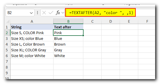
To make the formula case-insensitive, so it accepts the word-delimiter regardless of the letter case, we set the match_mode argument to 1:
=TEXTAFTER(A2, “color “, ,1)
That’s how to use the TEXTAFTER function to extract text after a specific character or word in Excel 365. I thank you for reading and hope to see you on our blog next week!


