Excel TOCOL function – convert range to single column
An easy way to transform an array or range into a column with the TOCOL function.
The ability to transpose data from columns to rows and in reverse has been in Excel for quite a while. But converting a range of cells into a single column was a tricky task to crack. Now, that’s finally changing. Microsoft has introduced a new function, called TOCOL, which can do an array-to-column transformation in a blink. Below is a list of tasks that this new function can easily solve.
Excel TOCOL function
The TOCOL function in Excel turns an array or range of cells into a single column.
This function has three parts, but you only need to use the first one.
TOCOL(array, [ignore], [scan_by_column])
- Array (required) – This is the range or array you want to turn into a column.
- Ignore (optional) – This option lets you decide if you want to ignore certain values. You can choose:
- 0 or omitted (default) – Keep all values
- 1 – Ignore blank cells
- 2 – Ignore error values
- 3 – Ignore both blanks and errors
- Scan_by_column (optional) – This controls how Excel scans the array:
- FALSE or omitted (default) – Scan by row, from left to right.
- TRUE – Scan by column, from top to bottom.
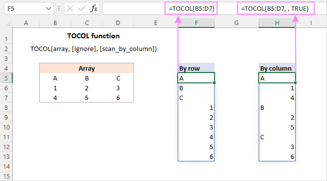
TOCOL availability
TOCOL is a new function, which is supported in Excel for Microsoft 365 (for Windows and Mac) and Excel for the web.
Basic TOCOL formula to transform range into column
The TOCOL function can be used with just one argument – the array. For example, if you have a block of cells with 3 columns and 4 rows, you can turn it into a single column with this formula:
=TOCOL(A2:C5)
You only need to enter the formula in one cell (like E2), and Excel will automatically fill the cells below it with the result. This is called a spill range in Excel.
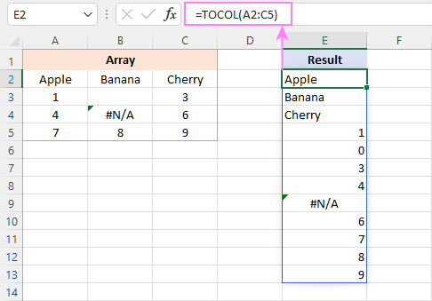
How this formula works:
Technically, the range A2:C5 is first converted into a two-dimensional array. Please notice the semicolon-separated rows and comma-delimited columns:
{“Apple”,”Banana”,”Cherry”;1,0,3;4,#N/A,6;7,8,9}
The TOCOL function scans the array from left to right and transforms it into a one-dimensional vertical array:
{“Apple”;”Banana”;”Cherry”;1;0;3;4;#N/A;6;7;8;9}
The result is placed in cell E2, from which it spills into the below cells.
How to use TOCOL function in Excel - formula examples
To better understand what the TOCOL function can do and how it can be useful, let’s look at a few example formulas
Transform array to column ignoring blanks and errors
As you saw in the earlier example, the basic TOCOL formula includes everything from the original range—even blank cells and errors.
In the result, blank cells are shown as zeros, which can be confusing—especially if your data also has real zeros. To fix this, you can tell Excel to skip blanks or errors using the second argument.
Here’s how:
- To skip blank cells:
=TOCOL(A2:C5, 1) - To ignore errors:
=TOCOL(A2:C5, 2) - To skip both blanks and errors:
=TOCOL(A2:C5, 3)
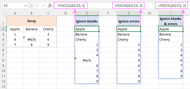
Scan array horizontally or vertically
By default, the TOCOL function scans the array across each row, from left to right. This happens when the scan_by_column part is left out or set to FALSE.
If you want Excel to read the values down each column instead, set this argument to TRUE (or 1). For example:
=TOCOL(A2:C5, , TRUE)
In both cases, the result will have the same number of values, but the order of those values will be different depending on how the array was scanned.
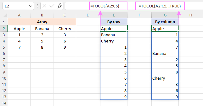
Combine multiple ranges into one column
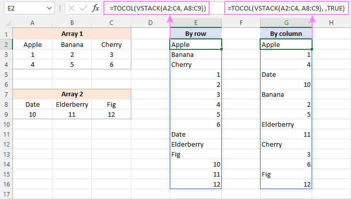
If you’re working with multiple ranges that aren’t next to each other, you can first combine them into one using the VSTACK function. Then, use TOCOL to turn the combined data into a single column.
For example, if your two ranges are A2:C4 and A8:C9, the formula looks like this:
=TOCOL(VSTACK(A2:C4, A8:C9))
This formula uses the default setting, so it reads the data row by row (left to right), and stacks everything into one column.
If you want to read the values column by column (top to bottom), use TRUE for the 3rd argument:
=TOCOL(VSTACK(A2:C4, A8:C9), , TRUE)
Keep in mind: in this case, Excel reads the entire stacked array—not each original range separately. So it will first take all values from column A, then column B, and so on.
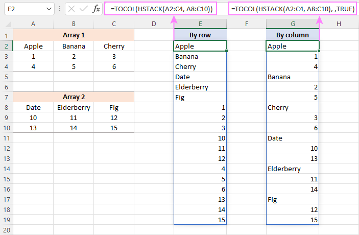
If you need to stack your ranges side by side (horizontally) instead of one below the other, use the HSTACK function instead of VSTACK.
- To join the arrays side by side and read them left to right (row by row), use this formula:
=TOCOL(HSTACK(A2:C4, A8:C10))
- To join the arrays side by side and read them top to bottom (column by column), use this one:
=TOCOL(HSTACK(A2:C4, A8:C10), , TRUE)
In both cases, the arrays are combined across, and TOCOL turns them into a single column, based on how you want to read the data.
Extract unique values from a multi-column range
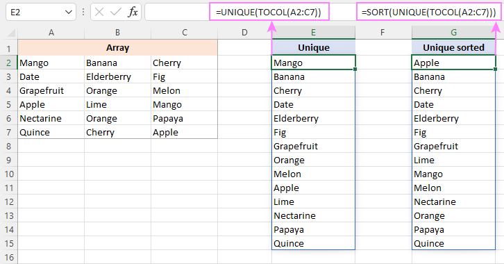
The UNIQUE function in Excel works well for finding unique values in a single row or column, and even for unique rows. But it doesn’t work directly on a range with multiple columns if you just want the individual unique values.
To fix this, use UNIQUE together with TOCOL.
For example, to get all the different values from the range A2:C7, use this formula:
=UNIQUE(TOCOL(A2:C7))
If you want to sort the results alphabetically, wrap the formula inside the SORT function like this:
=SORT(UNIQUE(TOCOL(A2:C7)))
That’s how you can use the TOCOL function in Excel 365 and alternative solutions in earlier versions to transform a 2-dimensional array into a single column. I thank you for reading and hope to see you on our blog next week!


