CHOOSECOLS function in Excel to get columns from array or range
This tutorial will teach you about a new Excel 365 function called CHOOSECOLS. It’s a dynamic array function that helps you pick certain columns from a larger set of data.
Imagine you’re working with a dataset that has hundreds or even thousands of columns. Some of these columns are more important than others, and you might want to look at those first. Excel 365 has a great tool for this. The CHOOSECOLS function lets you quickly pull out only the columns you need, so you can focus on the most useful information.
Table of Contents
Excel CHOOSECOLS function
The CHOOSECOLS function in Excel helps you pick and show certain columns from a group of cells (called a range or array).
Here’s how the function works:
- array – This is the group of cells you’re using.
- col_num1 – This is the number of the first column you want to get.
- col_num2, … – (Optional) You can add more column numbers if you want to pull out more columns.
Here’s an example of how the CHOOSECOLS function might look in your Excel sheet:

CHOOSECOLS function availability
Currently, the CHOOSECOLS function is available in Excel for Microsoft 365 (Windows and Mac) and Excel for the web.
How to use CHOOSECOLS function in Excel
CHOOSECOLS is a dynamic array function in Excel. This means it automatically works with arrays and fills in the results for you. You only need to type the formula in one cell (the top-left cell), and Excel will fill in the rest.
It will return as many columns as you ask for and match the number of rows from your original data. The result is called a “spill range” — a group of cells filled automatically by the formula.
To create a CHOOSECOLS formula in Excel, follow these steps:
- For array:
Give Excel the range of cells or values you want to work with. - For col_num:
Use numbers to tell Excel which columns to return:
- A positive number (like 1, 2, 3…) selects columns from left to right.
- A negative number (like -1, -2, -3…) selects columns from right to left.
- For multiple columns:
You can either add extra arguments for each column or provide an array constant with the column numbers.
For example, to get columns 2, 3 and 4 from the range A4:E19, the formula is:
=CHOOSECOLS(A4:E19, 2, 3, 4)
Alternatively, you can use a horizontal array constant such as {2,3,4} or a vertical array constant such as {2;3;4} to specify the column numbers:
=CHOOSECOLS(A4:E19, {2,3,4})
=CHOOSECOLS(A4:E19, {2;3;4})
All three formulas above will deliver the same result:

Sometimes, it’s easier to type the column numbers into separate cells and then use those cells in your formula. You can either refer to each cell one by one or use a range of cells all at once.. For example:
=CHOOSECOLS(A4:E19, G4, H4, I4)
=CHOOSECOLS(A4:E19, G4:I4)
This method gives you more flexibility — if you want to get different columns, just change the numbers in the cells. You don’t need to edit the formula at all.

Now that you know the essentials, let’s dive into the extras and explore a slightly more complex CHOOSECOLS formulas to handle specific scenarios.
Get last columns from range
If you want to pick columns from the end of a range, you can use negative numbers in the col_num part of the CHOOSECOLS function. This tells Excel to count columns from the right side instead of the left.
Here are some examples:
- To get the last column from the range A4:E19:
=CHOOSECOLS(A4:E19, -1) - To get the last two columns:
=CHOOSECOLS(A4:E19, -2, -1) - To get the last two columns but in reverse order:
=CHOOSECOLS(A4:E19, -1, -2)

Get every other column in Excel
To get every other column from a range, you can use CHOOSECOLS together with other Excel functions.
Below are two examples — one for getting odd-numbered columns and one for even-numbered columns.
- To get odd columns (like 1, 3, 5, etc.), use this formula:
=CHOOSECOLS(A4:E19, SEQUENCE(ROUNDUP(COLUMNS(A4:E19)/2, 0), 1, 1, 2)) - To get even columns (like 2, 4, 6, etc.), use this formula:
=CHOOSECOLS(A4:E19, SEQUENCE(ROUNDDOWN(COLUMNS(A4:E19)/2, 0), 1, 2, 2))
The screenshot below shows the first formula in action:

How this formula works:
Explanation: The CHOOSECOLS function returns every other column by using a list of odd or even numbers. This list is created by the SEQUENCE function, which generates numbers in order with a step of 2 (to skip every second column).
A detailed formula break-down:
The first step is to calculate how many columns to return. For this, we use one of these formulas:
ROUNDUP(COLUMNS(A4:E19)/2, 0)
or
ROUNDDOWN(COLUMNS(A4:E19)/2, 0)
The COLUMNS function counts how many columns are in your range. Since you want to take every other column, you divide that number by 2.
Then, depending on whether you want odd or even columns, you either round the result up or down.
- Use ROUNDUP to get odd columns
- Use ROUNDDOWN to get even columns
This rounding is important when your range has an odd number of columns—so the math works out correctly.
For example, if your range has 5 columns:
- Odd columns: ROUNDUP(5/2, 0) gives 3
- Even columns: ROUNDDOWN(5/2, 0) gives 2
That number is used as the first part (number of rows) in the SEQUENCE function.
- To get odd columns:
SEQUENCE(3, 1, 1, 2)
This gives you the numbers {1; 3; 5} - To get even columns:
SEQUENCE(2, 1, 2, 2)
This gives you the numbers {2; 4}
These arrays are passed into the CHOOSECOLS function, which uses them to pull out just the columns you want—either the odd or even ones.
Flip an array horizontally in Excel
To reverse the order of columns in an array (so they go from right to left), you can use CHOOSECOLS, SEQUENCE, and COLUMNS functions together like this:
=CHOOSECOLS(A4:D19, SEQUENCE(COLUMNS(A4:D19)) *-1)
As a result, the original range is flipped horizontally like shown in the image below:

How this formula works:
In this example, we use the SEQUENCE function to create a list of numbers that match the number of columns in the source array. To do this, we put COLUMNS(A4:D13) inside the rows part of the SEQUENCE function:
SEQUENCE(COLUMNS(A4:D19))
We don’t need to provide the other arguments (columns, start, step), so they will use their default values of 1. This makes SEQUENCE create a list of numbers like 1, 2, 3, …, up to n, where n is the total number of columns in the array.
To make the CHOOSECOLS function count columns from right to left, we multiply each number in the sequence by -1. This changes the list to negative numbers, like {-1; -2; -3}, which we then pass into the col_num part of CHOOSECOLS.
As a result, CHOOSECOLS will return the columns from the right side of the array:
CHOOSECOLS(A4:D19, {-1; -2; -3; -4})
Extract columns based on string with numbers
If the column numbers you want are given as a text string, you can use the TEXTSPLIT function to break the string into separate numbers using a divider (called a delimiter). Then, you can give this list of numbers to CHOOSECOLS to pick those columns.
Let’s say the column numbers are listed in cell H3, separated by a comma and a space. To get the columns of interest, use this formula:
=CHOOSECOLS(A4:E19, TEXTSPLIT(H3, “, “) *1)

Extract columns from multiple ranges
If you want to get specific columns from different ranges that aren’t next to each other, first use the VSTACK function to join all the ranges into one big range. After that, use CHOOSECOLS to pick the columns you want from this combined range.
For example, if you want to get columns 1 and 3 from the ranges A4:D8, A12:D15, and A19:D21, use this formula:
=CHOOSECOLS(VSTACK(A4:D8, A12:D15, A19:D21), 1, 3)

That’s how to use the CHOOSECOLS function in Excel to return particular columns from a range or array. Thank you for reading and see you on our blog next week!