Merge Cells in Excel
Merge cells is to combine multiple cells into one cell which can further be used for giving title to the report or header to the column. It helps to create clean reports format and clean document prints.
Why merging cells used in Excel?
If you work with data in Excel, you may find yourself in a situation where you need to merge cells in order to create a single, cohesive unit of information. For example, you may have a list of data that contains first and last names in separate cells, and you want to combine them into a single cell.
Fortunately, Excel makes it easy to merge cells.
Excel Shortcut - How to merge cells in Excel?
There are multiple ways to use shortcut for merging cells in Excel. Here are mostly used methods:
- Merge Cells: ALT H+M+M.
- Merge & Center: ALT H+M+C.
- Merge Across: ALT H+M+A.
- Unmerge Cells: ALT H+M+U.
Step by Step Guide to Merge Cells in Excel
Let’s quickly scroll down a bit more to understand the steps of How to Merge Cells in Excel.
Step 1
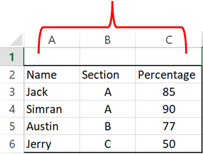
Select the cells you want to Merge with the help of mouse example A1 to C1.
or
Select the cell (A1), hold the Shift key and move the Right arrow key till cell C1. So this process will highlight the Range (A1 to C1) as displayed in below image:
SHIFT+ (→) Right Arrow Key for Row Selection
SHIFT+ (↓) Right Arrow Key for Column Selection

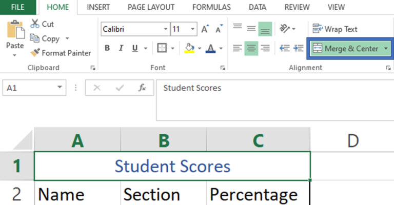
Step 2: Click on the Home tab and select Merge & Center Option as Highlighted in below image:
This will merge all cells through A1:C1 and will display it as one cell. See how “Student Scores” is displaying across A1:C1. This is called merging cells.
Also Merge cell option deletes the content of other cells and only display the content of first left or upper left cell.

If you want to align your text on the right side or left side, you may use alignment option to align text within merged cells
Disadvantageous of using Merge Cells in Excel
- It is quite difficult to copy and paste data in the merged cells.
- Post merging cells, data gets deleted from all the cells and only first cell data remain visible in the sheet i.e. First Left cell value or Upper Left cell value
Hope you liked this article. Please do comment your views on the same.
Download Practice File
Similar Topics
If you like to watch videos for learning Microsoft Advanced Excel, then you may click here and subscribe our channel


