VBA Code to Filter Data in Excel
VBA Code to Filter Data in Excel
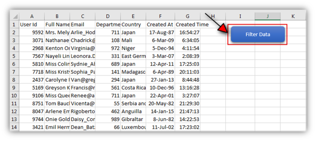
Here is an easy reference code which filters data in the sheet. In the code, we have filtered the data in three steps.
Step 1: Remove existing filter from the sheet (if any). This code ensures if there is already a filter applied then the same is removed first
Step 2: Apply filter on 5th column (E) of the data where Country is Japan
Step 3: Apply filter on 4th column (D) of the data where Department ID is 711
Method 1
					'This function can be used to filter data
Public Sub FilterData()

    'Reset/Remove filter from sheet
    Sheet1.AutoFilterMode = False

    'Apply first filter on 5th column (E) in the data where Country is Japan
    Sheet1.Range("A1:G" & Sheet1.Range("A10000").End(xlUp).Row).AutoFilter 5, "Japan"

    'Apply second filter on 4th column (D) in the data where Department ID is 711
    Sheet1.Range("A1:G" & Sheet1.Range("A10000").End(xlUp).Row).AutoFilter 4, "711"

End Sub
Method 2
					'This function can be used to filter data
Public Sub FilterData()

    'Reset/Remove filter from sheet
    Sheet1.AutoFilterMode = False

    'Apply first filter on 5th column (E) in the data where Country is Japan
    Sheet1.Range("A1:G" & Sheet1.UsedRange.Row).AutoFilter 5, "Japan"

    'Apply second filter on 4th column (D) in the data where Department ID is 711
    Sheet1.Range("A1:G" & Sheet1.UsedRange.Row).AutoFilter 4, "711"

End Sub
VBA Code to Filter Data in Excel, follow below steps:
- Open an Excel file
- Press Alt+F11
- Insert a Module (Insert>Module) from menu bar
- Paste the code in the module
- Now add a shape in Excel sheet
- Give a name to the shape like ‘Filter Data’
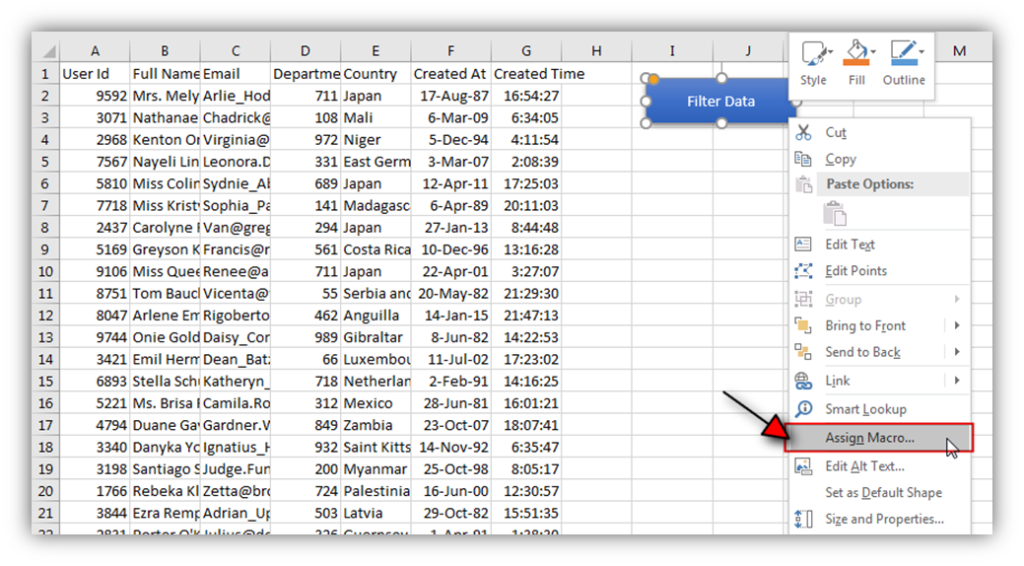
- Right click on the shape and select ‘Assign Macro…’
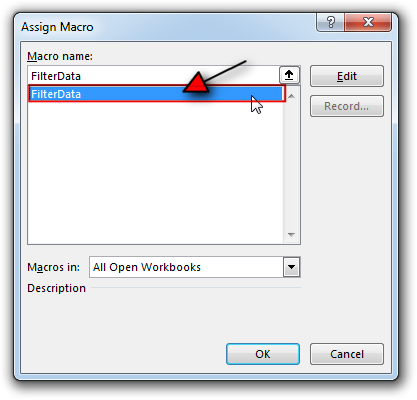
- Select ‘FilterData’ from the list and click on ‘Ok’ button
- Done, click on the shape to change the cell colors
Download Practice File
You can also practice this through our practice files. Click on the below link to download the practice file.
Hope You like this article. Please share this with your friends and colleagues.
Happy Reading