Here is an easy reference code which filters data in the sheet. In the code, we have filtered the data in three steps.
Step 1: Remove existing filter from the sheet (if any). This code ensures if there is already a filter applied then the same is removed first
Step 2: Apply filter on 5th column (E) of the data where Country is Japan
Step 3: Apply filter on 4th column (D) of the data where Department ID is 711
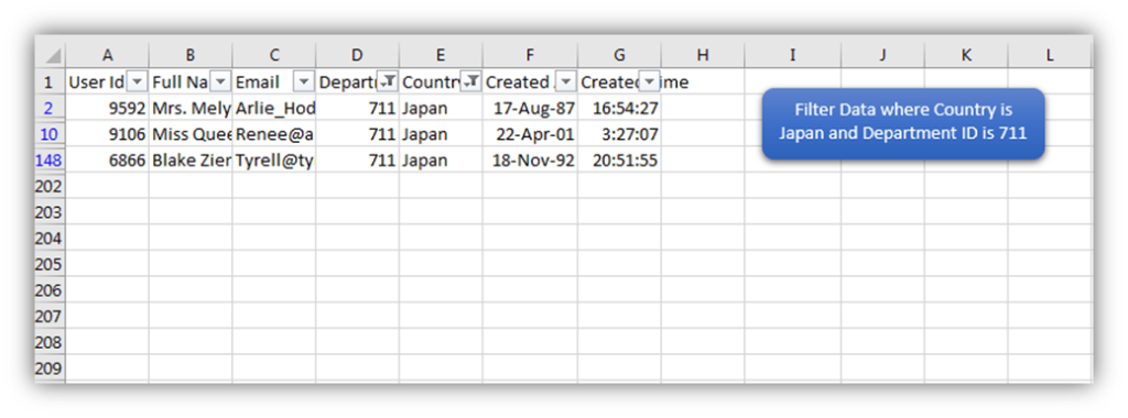
'This function can be used to filter data
 Public Sub FilterData()
     '
     'Reset/Remove filter from sheet
     Sheet1.AutoFilterMode = False
     '
     'Apply first filter on 5th column (E) in the data where Country is Japan
     Sheet1.Range("A1:G" & Sheet1.UsedRange.Row).AutoFilter 5, "Japan"
     'Apply second filter on 4th column (D) in the data where Department ID is 711
     Sheet1.Range("A1:G" & Sheet1.UsedRange.Row).AutoFilter 4, "711"
     '
 End Sub
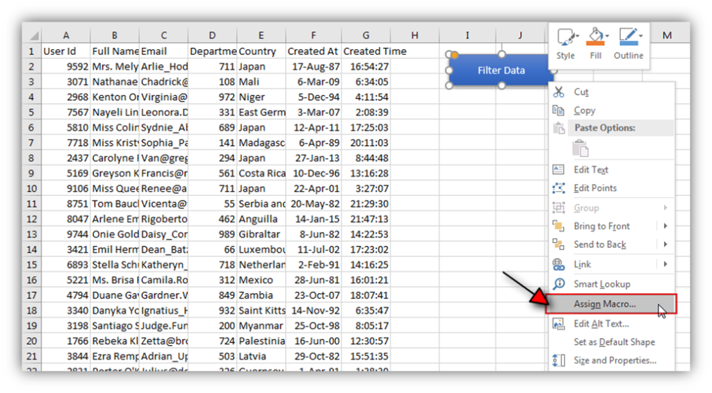
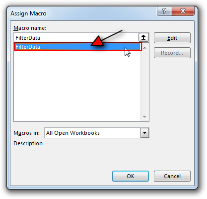
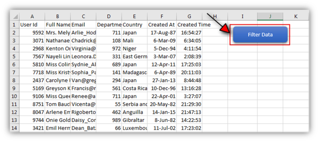
Hope You like this article. Please share this with your friends and colleagues.
Happy Reading

Want to learn how to unprotect Excel worksheet? Follow this simple guide to master this important skill in Excel. You can protect an Excel worksheet with or without a password. This helps keep your data…
How to Find Duplicate Files In excel using VBA? Yesterday I was working on my computer and cleaning the drives to make some more space. I was surprised to see so many files saved at…

VBA Tools To Create Folders In VBA, you can use MkDir function to create folders in your system or shared drive. To make your work simple, we bring a free Excel VBA tool to create…
This step-by-step tutorial empowers you to leverage Power Query’s robust filtering capabilities. Learn to filter by date, text, numbers, and more, streamlining your workflow and unlocking deeper insights from your data. Watch now and elevate your Excel expertise!

How to Export Access Data to Excel using VBA Code? Creating a VBA tool in MS Access is always better as compare to MS Excel. MS Access provides better user interface and ability to handle…

This Excel VBA Code helps to Get User Name. Here is an example environ(username) or Application.username.This macro gets the username from active directory.