FIND function is used to locate the position of text, or character in an available string.
FIND Function has argument two required arguments i.e. find_text, within_text and one optional argument i.e. [start_num]. If no value is provided in [start_num] argument then function will take the Default value i.e. 1
=FIND(find_text, within_text, [start_num])
find_text argument, is used to give text, character or cell reference that is required to find
within_text argument, is used to give the cell reference from which text (i.e. find_text value ) to be searched
[start_num] is optional argument and is used to specify the character from which search should start. By default, the first character is 1, however if you want search should be started from 2nd find_text value then it should be position of 2nd find_text value and so on..
Here we have some examples, where:
– “Column A” has various strings,
– “Column B” shows the sample formula that is applied,
– “Column C” shows the output of the function and
– Explanation is provided in “Column D

– Output in Cell “C2” i.e. “6” is showing that the character “u” is available at “once upon” and “u” has 6th position.
– Output in Cell “C3” i.e. “13” is showing that the character “T” is available at “Tree” and has 13th position. Also note that character “t” is ignored in “there”
– Output in Cell “C4” i.e. “8” is showing that the character “t” is available at “tree” after ignoring character “t” at “that”.
– Find function is case sensitive, means it will only search “t” for text “the” and not with “The”. If you want to find value without case sensitive, then try “SEARCH” Function
– Find function will not work with Wild characters i.e. asterisk (*), question mark (?)
– Function should give output in “General” format, however if output is not as per the desired format then we need to change the cell format to “GENERAL”.
– If function parameters are not correctly applied in the function, then it will give output as “#VALUE!” (Error).
Don’t forget to leave your valuable comments!
If you liked this article and want to learn more similar tricks, please Subscribe us

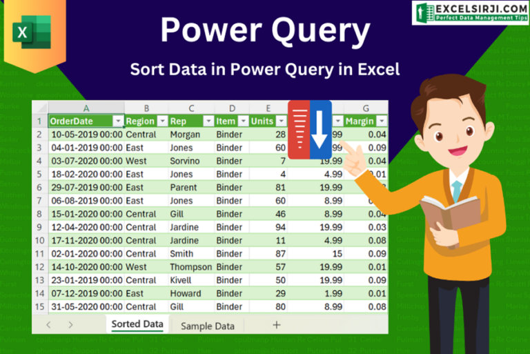
This article unveils the magic of Power Query, a built-in Excel tool that simplifies data organization. Learn how to sort by single or multiple columns, create layered sorts for complex needs, and even reverse your data order entirely. Power Query puts you in control, transforming your data into a well-structured format for effortless analysis.

The tutorial explains how to use the CHOOSE function in Excel, showing you the basics and some interesting examples. While CHOOSE might seem simple on its own, when you combine it with other functions, it can be powerful. Essentially, the CHOOSE function helps you pick a value from a list based on its position. The tutorial also covers some advanced ways to use CHOOSE that you might find very useful.

This quick tutorial explains the basics of external references in Excel and shows how to reference another sheet or workbook in your formulas.

Calculate Percentage in Excel Calculate Percentage in Excel :-The term “per cent” comes from the Latin per centum, meaning “by the hundred.” A percentage is a way to show a part of something out of…

This tutorial explains how to use the new TEXTSPLIT function in Excel 365 to break text into separate parts using any symbol or space you choose. Sometimes, you may need to split text in Excel….

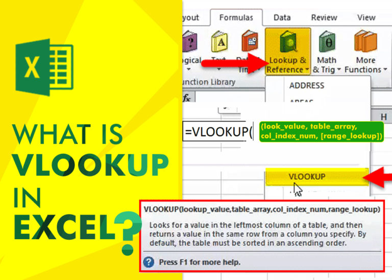
An ultimate guide for basic user to understand Excel Vlookup function. VLOOKUP is a vertical lookup which helps the user to extract the values from other columns (leftmost) basis on matching column string.