While working with Microsoft Excel, did you get a situation where you need to extract the characters from a string? I believe most of your answers are YES. In the said scenario “MID” function will help you to find the solution. We will be learning the Microsoft Excel “MID” in details, so stay with us and continue reading…
MID function is used for extracting the mid characters from the available string. The output of the function returns the extracted characters in new cell.
Function should give output in “General” format, however if output is not as per the desired format then we need to change the cell format to “GENERAL”.
MID Function has argument three arguments i.e. text, start_num and num_chars where we need to give the cell references and parameters. We can give the parameters as per the requirement by following the “ , “ (i.e. Comma) as separator.
If parameters are not separated by “ , “ (i.e. Comma) or quotation mark is/are missing or any other function error then it will give output as “#VALUE!” (Error). So always ensure that function parameters are used to get the appropriate results/output.
=MID(text,start_num,num_chars)
Excel MID Function has three compulsory parameters, i.e, text, start_num, num_chars
The MID function in Excel is very simple and easy to use. Let us understand the working of the MID function in Excel by some MID formula example.
We will be following MID function as follows:
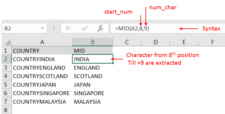
– “text argument”: “A2” is the cell reference from which characters should be extract
– “start_num argument”: “8” is the 8th character from string should be extracted
– “num_char argument”: “9” is the total number of characters from the string should be extracted starting from 8th character

Explanation: we can see ignored “COUNTRY” has total 7 character that is why character 8th position is mentioned in “start_num argument”. Also, total 9 characters are required after 8th that is why “9” is mentioned in “num_char argument” i.e. till 8+9 = 17 characters
Hope you learnt this Function,
Don’t forget to leave your valuable comments!

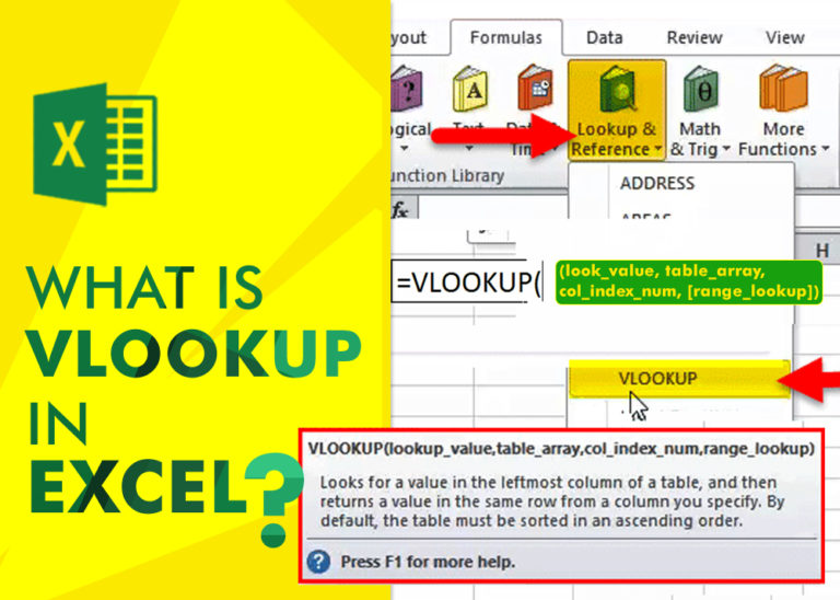
An ultimate guide for basic user to understand Excel Vlookup function. VLOOKUP is a vertical lookup which helps the user to extract the values from other columns (leftmost) basis on matching column string.

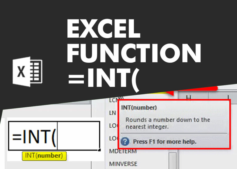
INT function is used to round down the numeric value to nearest integer. INT Function has one required argument i.e. number.

Calculations With Date In Excel Dates function also be used to subtract the Year, Month and Days from the existing dates. Sometimes we need to subtract specific period from the date. In case you are…

This guide shows how to use the nested IF function in Excel to check several conditions. You will also learn about other functions that can be to use than a nested formula.
When you want to make decisions in Excel, you often use an IF formula. It checks if something is true, then gives one result if it is and another result if it isn’t. If you need to check more than one thing, you can put many IFs inside each other.
Although using multiple IFs is common, it’s not the only way to check several conditions in Excel. This guide will introduce you to some easier and useful alternatives.

Excel Function- WORKDAY.INTL WORKDAY.INTL function is an advanced version of WORKDAY function with additional advantage of “Custom weekend options” For Example, with WORKDAY function weekends are treated as “Saturday and Sundays” however if you need…

Do you work with lots of data in Excel? Sorting, summarizing, and organizing information can take time. You may have used features like outlines, subtotals, or pivot tables before. But now, there’s an even simpler…