=SUBSTITUTE(text,old_text,new_text,[instance_num])
Text argument [Required] is used to give the cell reference in which value to be searched
old_text argument [Required], is used to give the specific text or cell reference, to be substituted
new_text argument [Required], is used to give the specific text or cell reference that you want to substitute in old_text
instance_num argument [Optional], is used to give the occurrence number that you want to substitute
Here we have an example, where “Column A” has various values and are required to substitute year “2018” with “2019”. Output of the function returns value in ”Column B” and explanation is also provided.
We will be following SUBSTITUTE function as follows:
– text argument value “A2” shows the cell reference in which “2018” is to be searched
– old_text argument value “2018” shows that “2018” should be replaced in “A2” cell
– new_text argument value “2019” shows the substituted value
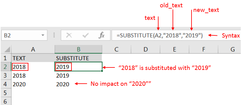
– Value in cell “B2” shows that “2018” in cell “A2” is substituted with “2019”
– Value in cell “B4” shows that cell “A2” did not have “2018” that is why text is not substituted and function returns original value of cell “A2” as output
Here we have another example, where “2018” should be replaced with “2019” but ONLY SECOND OCCCURRENCE. Output of the function returns value in ”Column B” and explanation is also provided.
We will be following SUBSTITUTE function as follows:
– text argument value “A2” shows the cell reference from which “2018” is to be searched
– old_text argument value “2018” shows that “2018” should be searched in “A2” cell
– new_text argument value “2019” shows the substituted value
– instance_num argument value “2” shows only 2nd occurrence to be substituted and there should no impact on other values.
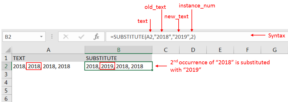
– Value in cell “B2” shows that “2018” in cell “A2” is substituted with “2019” but only 2nd occurrence and there is no impact on
– Spaces available in a string is counted as characters
-Value in instance_num argument should NOT be negative
– If value in old_text argument is not searched in text argument cell, function will return value of text argument cell
– If cell reference or parameters are not correctly provided in the function, then it will give output as “#VALUE!” (Error).
– Function should give output in “General” format, however if output is not as per the desired format then we need to change the cell format to “GENERAL”.
Hope you learnt this Function,
Don’t forget to leave your valuable comments!
If you liked this article and want to learn more similar tricks, please Subscribe us or follow us on Social Media by clicking below buttons:

TEXT function is used to change the formatting or appearances of the text. There are various types of formatting available.

The Article of DATEVALUE explains how to use Excel functions to change text into dates and numbers into dates. It also shows how to convert text strings into dates without using formulas. You’ll also learn…
This guide will show you quick and easy methods to find the number of days between dates in Excel.
Do you need to know how many days are between two dates? Maybe you want to find out the days between today and a date in the past or future, or just count the working days between two dates? Whatever you need, one of the examples below will help you find the solution
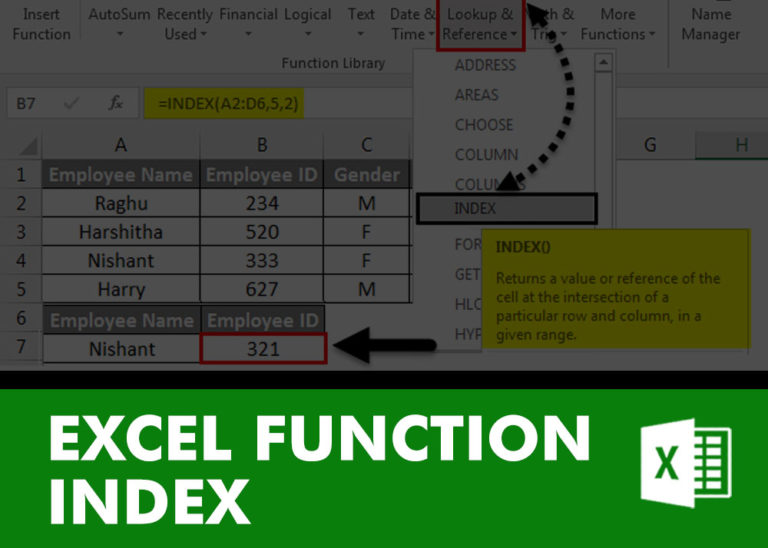
INDEX function is used to get the value from a cell range or table, function returns the value from a table where row and column intersect with each other.
SUMPRODUCT function performs multiplication of numbers within arrays and then sum the values SUMPRODUCT function has array1, 2.. arguments.
ROWS function is used to get the total count of rows in an array or in cells range in an excel worksheet.