INDEX function is used to get the value from a cell range or table, function returns the value from a table where row and column intersect with each other.
INDEX function has two Required arguments i.e. array, row_num and one Optional argument i.e. [column_num]. [column_num] argument is optional only if array argument contains one column.
=INDEX(array,row_num,[column_num])
array argument is used to give the cell range from which you want to get value
row_num argument is used to give the row number from which value is required
[column_num] argument is used to give the column number from which value is required. If array argument only has only one column, then [column_num] argument is optional
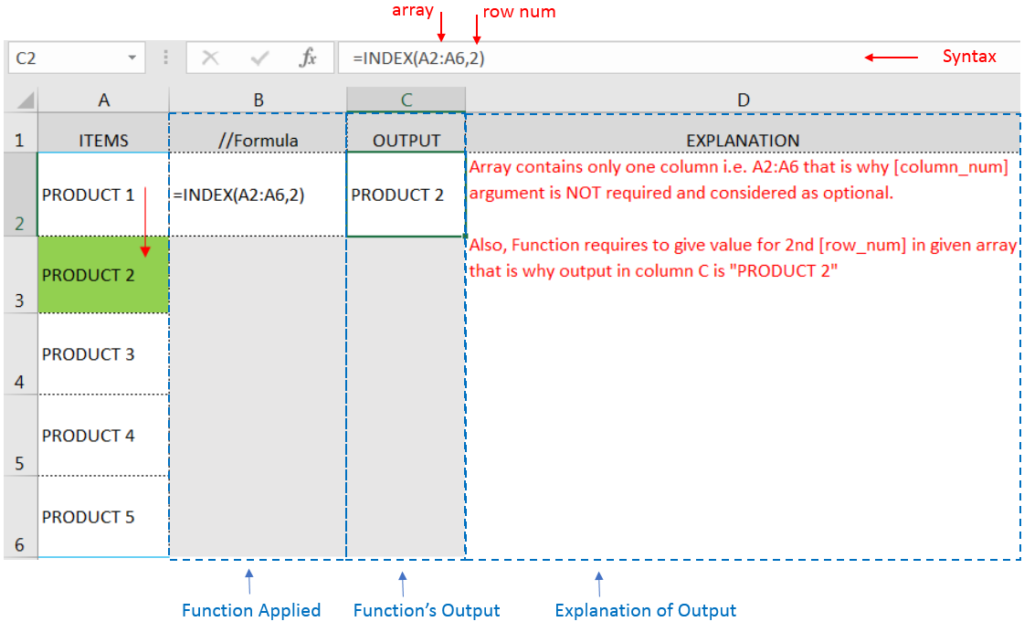
Here we have one example, where:

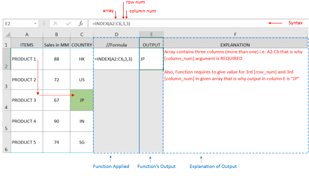
Here we have another example, where:

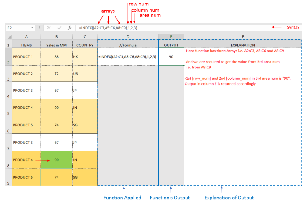
Here we have another example, where:

– If cell reference is not correctly provided in the function, then it may give output as Error.
– If output of the function is not as per the desired format then you may change the cell format to “GENERAL”
Hope you learnt this Function,
Don’t forget to leave your valuable comments!
If you liked this article and want to learn more similar tricks, please Subscribe us.

What is COUNTIFS in Excel? The Microsoft Excel COUNTIFS function counts the number of cells in a range, that meets a single or multiple criteria and adjacent or non-adjacent. As a Statistical function of Excel,…

Excel Function REPLACE REPLACE function is used to replace the existing text from a specific location in a cell to New Text. REPLACE Function has argument four arguments i.e. old_text, start_num, num_chars and new_text. We need to give the…

SUMIF function is used to get the “total sum” for number of times the criteria across range is met. SUMIF Function has two required arguments.

RIGHT function is used for extracting the “Right Most” characters from the available string in Microsoft excel. Function returns value to new string.

SUBSTITUTE function is used to substitute the existing old text to new text.

The tutorial explains what the Compound Annual Growth Rate (CAGR) is and shows how to create a clear and easy-to-understand formula for calculating CAGR in Excel.