Merge cells is to combine multiple cells into one cell which can further be used for giving title to the report or header to the column. It helps to create clean reports format and clean document prints.
If you work with data in Excel, you may find yourself in a situation where you need to merge cells in order to create a single, cohesive unit of information. For example, you may have a list of data that contains first and last names in separate cells, and you want to combine them into a single cell.
Fortunately, Excel makes it easy to merge cells.
There are multiple ways to use shortcut for merging cells in Excel. Here are mostly used methods:
Let’s quickly scroll down a bit more to understand the steps of How to Merge Cells in Excel.
Step 1
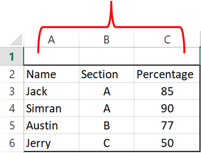
Select the cells you want to Merge with the help of mouse example A1 to C1.
or
Select the cell (A1), hold the Shift key and move the Right arrow key till cell C1. So this process will highlight the Range (A1 to C1) as displayed in below image:
SHIFT+ (→) Right Arrow Key for Row Selection
SHIFT+ (↓) Right Arrow Key for Column Selection

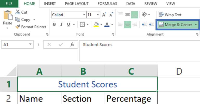
Step 2: Click on the Home tab and select Merge & Center Option as Highlighted in below image:
This will merge all cells through A1:C1 and will display it as one cell. See how “Student Scores” is displaying across A1:C1. This is called merging cells.

If you want to align your text on the right side or left side, you may use alignment option to align text within merged cells
Hope you liked this article. Please do comment your views on the same.
If you like to watch videos for learning Microsoft Advanced Excel, then you may click here and subscribe our channel

“NETWORKDAYS” function is very helpful feature in the Microsoft excel to calculate the working days from a particular period excluding “Saturday and Sundays”. NETWORKDAYS function subtract the Start Day from the End Date provided.

In this tutorial you’ll learn how to use the TEXTBEFORE function in Excel to quickly get the text before a specific character or word.In older versions of Excel, this was more difficult. You had to…

SEARCH function is used to find “position of character or text” in an available cell and this function is NOT case sensitive.

MIN function is used to get the smallest number in range or list of values.MIN function has one required i.e. number1 and optional argument i.e. [number2]

MID function is used for extracting the mid characters from the available string. The output of the function returns the extracted characters in new cell.

ROUND function rounds the number value to nearest digit mentioned in argument.
ROUND function has two required arguments i.e. number and num_digits