How to use Power Query in Excel – practical examples
This tutorial shows how to use Power Query in Excel with real-life examples.
In the last article, we talked about the basics of Power Query. Now, we’ll look at how you can use it in everyday tasks. Below, you’ll find several examples to help you understand how Power Query works in real situations.
These examples start from the point where you already have your data loaded into the Power Query Editor. If you haven’t done that yet, don’t worry — you can go back to our previous tutorial to learn how to load your data.
To help you follow along, we’ve also made a sample Excel workbook that you can download at the end of this post. Let’s get started and see how Power Query can help with your data!
Table of Contents
What is Power Query In Excel?
Power Query in Excel is a data connector and transformation tool that allows users to import, shape, and combine data from various sources into Excel. It’s a powerful feature for cleaning, preparing, and preparing data for analysis.
Trim and clean
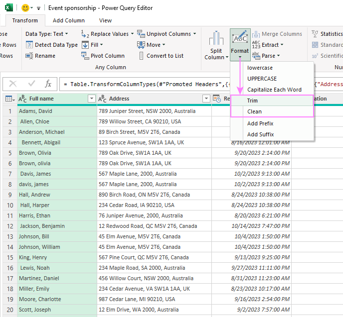
To remove any leading or trailing spaces, or any other unwanted characters, you can use the Trim and Clean functions. Select the columns you want to clean up, go to the Transform tab > Text Column group and click Format > Trim or Clean.
Remove duplicate rows
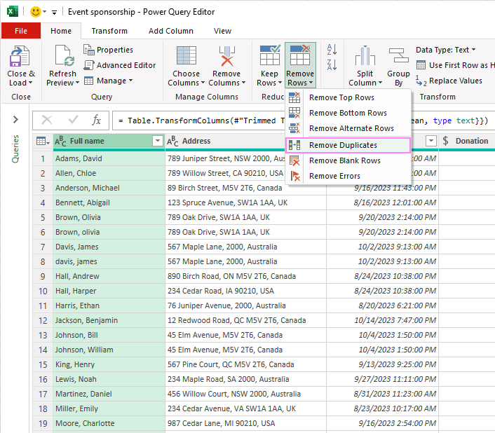
To eliminate duplicate rows in your data, Power Query offers the Remove Duplicates function. Select the column(s) you want to check for duplicates, then go to the Home tab, and click on Remove Rows > Remove Duplicates.
Remove duplicates case-insensitive
Please note that the “Remove Duplicates” feature will only remove rows that are exactly the same in every way, including how the letters are capitalized. If you want to remove duplicates without considering letter case, you’ll need to change the M code for the query. Here’s how to do that:
- First, remove the case-sensitive duplicates as usual. Or, you can right-click the column you want to clean up and choose “Remove Duplicates” from the menu.
- In the Formula Bar, add Comparer.OrdinalIgnoreCase to the second part of the Table.Distinct function to ignore letter case.
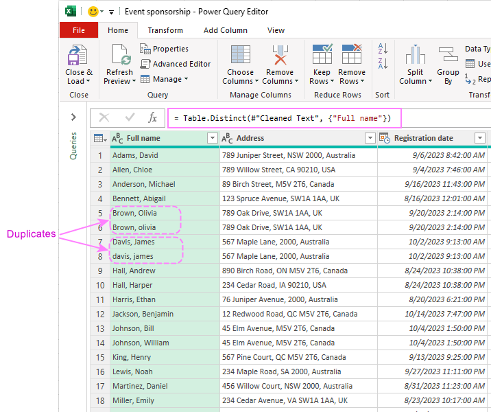
For example, after removing the duplicates normally, the Table.Distinct function looked like this:
=Table.Distinct(#”Cleaned Text”, {“Full name”})
This removed all rows where the names in column A were exactly the same, but it left some rows where the names had different letter cases, as shown in the screenshot below.
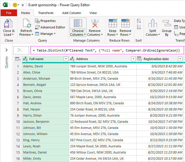
To fix this issue, you can add the Comparer.OrdinalIgnoreCase criterion to the function like this:
=Table.Distinct(#”Cleaned Text”, {“Full name”, Comparer.OrdinalIgnoreCase})
This will eliminate all the rows containing duplicates in column A, ignoring the letter case.
Users with advanced Excel skills can do this operation in the Advanced Editor by changing the Removed Duplicates line to this format:
Table.Distinct(PreviousStep, {“ColumnName”, Comparer.OrdinalIgnoreCase})
Change data type
If the data you imported doesn’t look quite right, don’t worry — you can quickly fix the format.
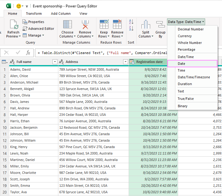
For example, in our sample data, the Registration Date column shows both the date and the time. If you only want to see the date, you need to change the column’s data type from Date/Time to just Date. There are two easy ways to do this:
- Go to the Home tab and choose Data Type > Date from the ribbon.
- Or, right-click the column header and select Change Type > Date from the menu.
Custom date format
Power Query uses the default date format based on your region settings. If you want to show dates in a different (custom) format, you can use the DateTime.ToText function. Just follow these steps:
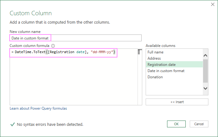
- Go to the Add Column tab and click Custom Column in the General group.
- In the window that pops up, type a name for your new column, like Date in custom format.
- In the formula box, use the DateTime.ToText function with two parts:
- The first part is the original date column.
- The second part is the format you want, like “dd-MMM-yy” (which shows dates like 18-Apr-25).
- To add the date column, select it from the list on the right and click Insert, or just double-click it.
- Then, type the format you want inside double quotes.
Your final formula should look like this:
=DateTime.ToText([Registration date], “dd-MMM-yy”)
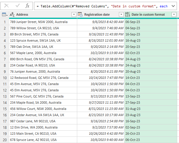
- Click OK, and a new column will appear showing the date in your custom format.
The formula bar will show the complete formula in the M language, which will look something like this:
=Table.AddColumn(#”Previous step”, “Date in custom format”, each DateTime.ToText([Registration date], “dd-MMM-yy”))
By changing the data type, you can format the values in a more suitable way for your analysis. Similarly, you can change other columns to different data types, such as text, number, or currency, depending on your needs.
Split column
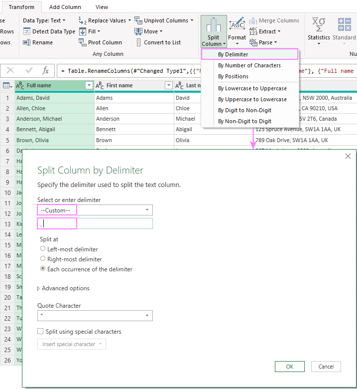
To split a column into two or more parts using a specific character (called a delimiter), you can use the Split Column feature. For example, if you want to split a Full Name column into First Name and Last Name, here’s what to do:
- Select the Full Name column.
- Go to the Transform tab. In the Text Column group, click Split Column > By Delimiter.
- Choose the character that separates the names (called a delimiter). For example, if names are separated by a comma and space, choose Custom and type , in the box.
- Choose how you want to split the column:
- Left-most delimiter: splits at the first comma.
- Right-most delimiter: splits at the last comma.
- Each occurrence: splits at every comma. If there’s only one comma in each cell, any option will work. But if there are more, choose carefully.
- Click OK when you’re done.
- Finally, right-click the new column headers and choose Rename to give them clear names, like First Name and Last Name.
Extract values into a new column
If a column in your data has long text with different parts, you might want to pull out just one part into a new column.
For example, let’s say you want to get the country name from the Address column. Here’s how to do it:
- Select the column that has the information you want to extract.
- Go to the Add Column tab, click Extract, and choose the option that fits your case.
– In our example, the country names come after a comma, so we pick Text After Delimiter.
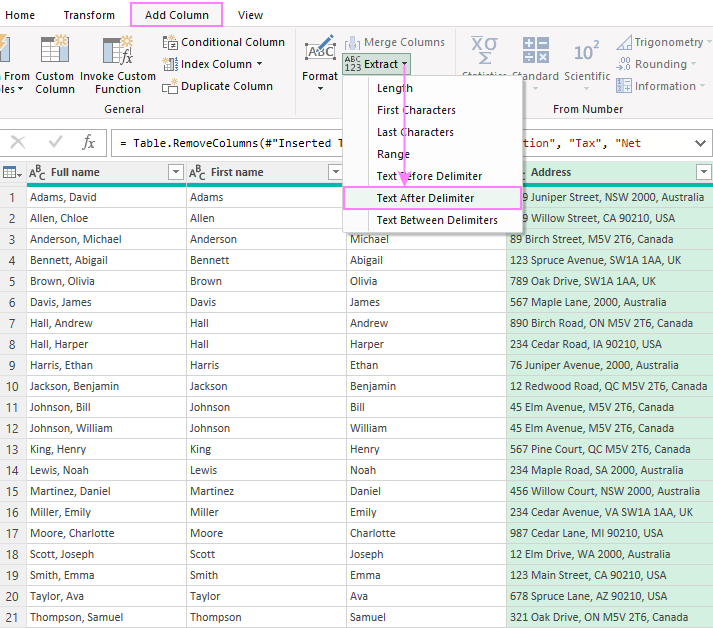
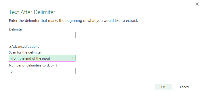
- In the dialog box that pops up, enter the delimiter (a comma and a space “, ” in our dataset).
- Expand the Advanced option section and choose to scan for the delimiter from the end of the input, as the country name comes after the last comma in a cell. If you need to extract a value from the middle of the string, indicate how many delimiters to skip.
- When done, click OK.
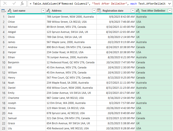
A new column with the extracted values will be added to the end of the table, and you can move it to any position you want by dragging the column header.
Add column from example
When your data is messy or incomplete, the usual Split and Extract tools might not work well.
For example, imagine the Address column has country names separated by different symbols like commas, spaces, or vertical bars (|). In this case, you can use a smart Power Query feature that lets you give an example — similar to Excel’s Flash Fill.
Here’s how to create a new column using an example:
- Select the column with the data you want to work with (like the Address column).
- Go to the Add Column tab and click Column from Examples > From Selection.
- In the first row of the new column, type the correct country name that matches the first address.
- Power Query will try to guess the pattern and fill in the rest of the column for you.
- If some results are blank or wrong, type more correct examples in the next rows until it gets everything right.
- Once you’re happy with the results, press Ctrl + Enter to save the changes.
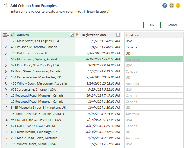
You will now have a new column that extracts the country names from the addresses.
Replace missing values
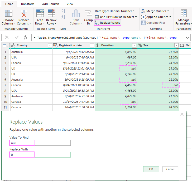
In Power Query, replacing missing values, often represented as null, is a straightforward process:
- Select the column(s) where you want to handle missing values.
- On the Home tab, in the Transform group, click Replace Values.
- In the Replace Values dialog box, fill in two boxes:
- Value To Find: null
- Replace With: enter the replacement value corresponding to your data type (e.g., “0” for numeric columns or “N/A” for text columns).
- Click OK, and Power Query will apply the replacement to all the selected columns.
Add conditional column
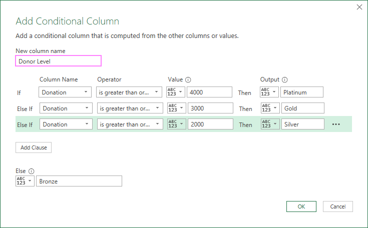
To add a new column based on conditions using the data in your existing columns, you can use the Add Conditional Column feature. For example, if you want to add a column that shows a donor level based on the donation amount, here’s how to do it:
- Select any column in your data.
- Go to the Add Column tab and click on Conditional Column.
- In the box that appears, type Donor Level as the name for your new column.
- Then, set up the following rules:
- If Donation is greater than or equal to 4000, then assign Platinum.
- If Donation is greater than or equal to 3000, then assign Gold.
- If Donation is greater than or equal to 2000, then assign Silver.
- Else, assign Bronze.
- Click OK to create your new column.
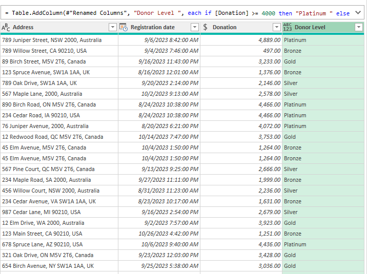
This feature is similar to writing a nested IF statement in Excel, but it’s a lot easier and more convenient to use.
By default, the new conditional column will appear at the end of your dataset, and you can drag it to any position you want.
Replace or remove errors
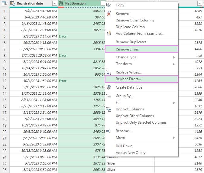
Power Query makes it easy to fix errors in your data without needing complex formulas or VBA code. To clean up errors in your dataset, just follow these steps:
- Select the column where you want to fix the errors.
- Right-click the column header.
- In the menu that appears, you’ll see two useful options:
- Remove Errors – This deletes all rows that have errors in the selected column. Be careful, because this also removes the data in those rows.
- Replace Errors – This lets you choose what to show instead of the error.
- For number columns, type a number (like 0) to replace the error.
- For text columns, you can type any text or even leave it blank.
Group and aggregate
To summarize or group your data, Power Query has a helpful tool called Group By.
For example, if you want to find the total donation amount by Country and Donor Level, here’s how to do it:
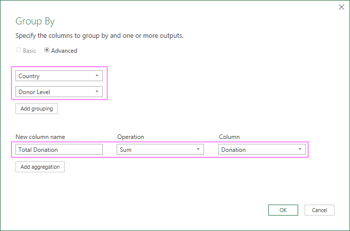
- Go to the Home tab, and in the Transform group, click Group By.
- In the window that appears, choose Advanced.
- Then fill out the options like this:
- Under Group by, select Country and Donor Level.
- Under New column name, type Total Donation.
- Under Operation, choose Sum.
- Under Column, select Donation.
- Click OK, and Power Query will group your data and show the total donations for each country and donor level.
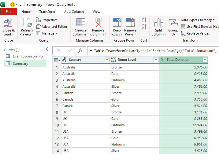
As a result, a new table will be created displaying the grouped and aggregated data. If needed, you can sort the table by one or more columns: right-click the filter arrow next to the column name and choose either to sort ascending or descending.
In this example, we get a summary of total donation amounts based on both country and donor level.
That’s how to use Power Query in Excel. Now that you know the basics, go ahead and unlock more data transforming secrets to impress your boss, colleagues, and clients with your data mastery 🙂


