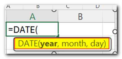


When you work with dates in Excel, the DATE function is crucial to understand. The reason is that some other Excel functions may not always recognize dates when they are entered as text. Therefore, when you do calculations involving dates in Excel, it’s best to use the DATE function to input dates. This helps ensure that your calculations give the right results.
Now while looking at above Formula, there are four parameters which are described as below:
This argument is used to denote or get the year from the serial numbers. It is advisable to use the four digits while using arguments for “Year”.
For Example: If you enter below formula
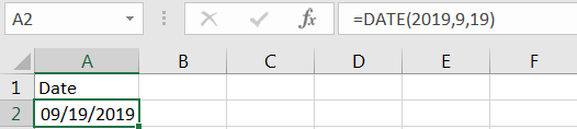
Syntax: =Date(2019,9,19) will give result to 09/19/2019
Lorem ipsum dolor sit amet, consectetur adipiscing elit. Ut elit tellus, luctus nec ullamcorper mattis, pulvinar dapibus leo.
And If you write the above formula as below:
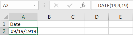
Syntax: =Date(19,9,19) will give result to 09/19/1919
In Excel, when you enter only two digits for the year, Excel interprets it based on its calendar starting from the year 1900. This can lead to incorrect results because Excel might convert ’19’ to 1919 (1900 + 19). Therefore, it’s important to enter the full year (four digits) to avoid such issues.
Therefore, it is advisable to use the correct syntax with four digits to ensure accurate results.
The month argument in Excel’s date functions represents the numeric value for the month, ranging from 1 to 12. If a negative number or a number greater than 12 is used, Excel adjusts it by adding or subtracting years accordingly.
For Example: If you enter below formula
Syntax: =Date(2019,9,19) will give result to 09/19/2019
So if you write this formula as below:
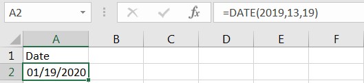
Syntax: =Date(2019,13,19) will give result to 01/19/2020
Here we mentioned “13” in the month, that is more than 12. In this case Microsoft excel will add the month and adjust the year. So adding 12+1 (i.e. December + 1 month) will be January and year would be changed to next year i.e. from 2019 to 2020
And if you write this formula like below:
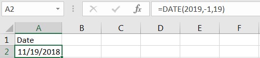
Syntax: =Date(2019,-1,19) will give result to 11/19/2018
Here we mentioned “-1” in the month. In this case Microsoft excel will deduct one month from the year and will provide the output. So, adjusting (2019 – 1 month) will be November and year would be changed to previous year i.e. from 2019 to 2018
This argument is used to denote or get the Day from the serial numbers. It is a numeric number starts from 1 to 31. If any negative or more than 31 numbers are used in function, then days would be adjusted from month and year.
For Example, if you write this formula:
Syntax: =Date(2019,9,19) will give result to 09/19/2019
So if you write this formula as:
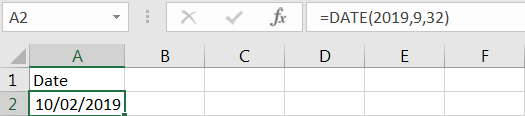
Syntax: =Date(2019,09,32) will give result to 10/02/2019
Here we mentioned “32” in the month, that is 2 additional days of 30 days in September. In this case Microsoft excel will add the days to next month. So, adding 30+2 (i.e. 30th September + 2 days) will be 2nd October and output will be 10/02/2019 (i.e. 2nd October 2019)
Now if you write this formula as
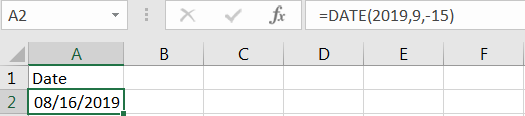
Syntax: =Date(2019,09,-15) will give result to 08/16/2019
When using “-15” for days in Excel, it subtracts 15 days from the given month. For example, adjusting from September by 15 days brings you to August 16th, resulting in the output 08/16/2019, which represents August 16th, 2019.
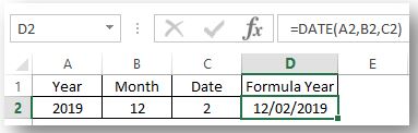
Here you may also link any of the above argument with any cells in excel to drive the formula on the basis of variables. So if your data is like below:
The formula in cell D2 uses the Date function linked to cells A2, B2, and C2. This makes it dynamic, allowing you to use the function with different values to create various dates. I hope you found this article helpful!
Please comment and share your valuable feedback or if you have any questions.

https://youtu.be/HmJL_y93pAs WEEKNUM function helps to calculate the week number of the given date in a year. It considers 1st January as first week by default and through the output for the given input date. Syntax:…
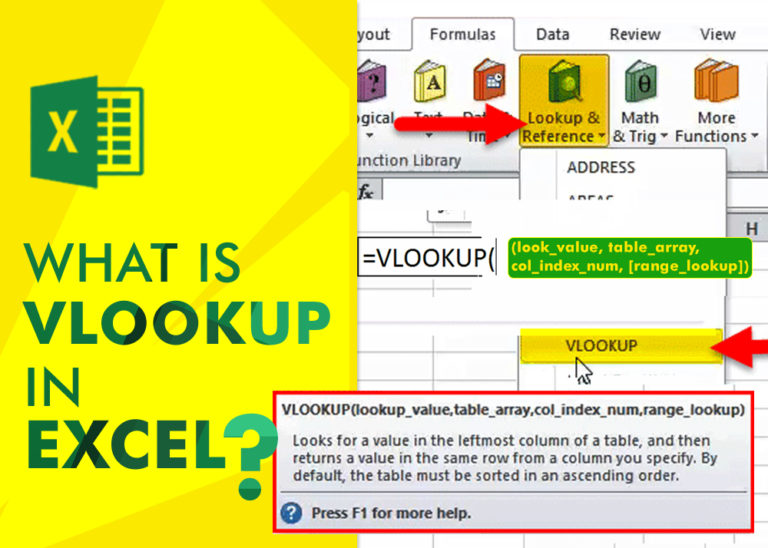
An ultimate guide for basic user to understand Excel Vlookup function. VLOOKUP is a vertical lookup which helps the user to extract the values from other columns (leftmost) basis on matching column string.

SUBSTITUTE function is used to substitute the existing old text to new text.

LEFT function is used for extracting the “Left Most” characters from the available string. The output of the function returns the extracted characters in new cell

SUMPRODUCT function performs multiplication of numbers within arrays and then sum the values SUMPRODUCT function has array1, 2.. arguments.

SEARCH function is used to find “position of character or text” in an available cell and this function is NOT case sensitive.
One Comment