
What is VLOOKUP in Excel?
How to use VLOOKUP in Excel?
Anyone who wants to get expertise in Excel, VLOOKUP is an essential function for those which can easily make you awesome in excel.
There are two kind of lookups in excel one is VLOOKUP and second is HLOOKUP. Both works on same methodology with small difference that VLOOKUP works vertically (in Columns) and HLOOKUP works horizontally (in Rows). That’s why these are called Vertical Lookups and Horizontal Lookups respectively.
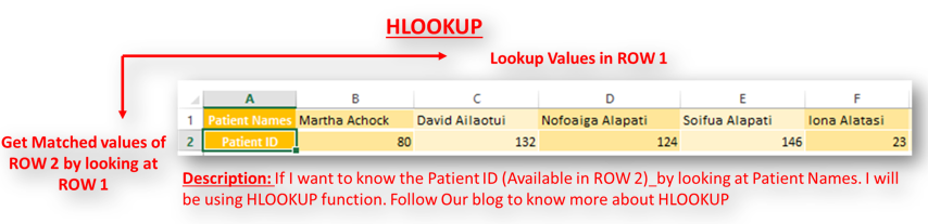
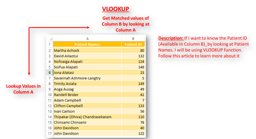
Here we are going to talk about VLOOKUP. There are many ways to use VLOOKUP which we will discuss with different methods and examples. Please follow our blog to become an expert of VLOOKUP
VLOOKUP STARTER
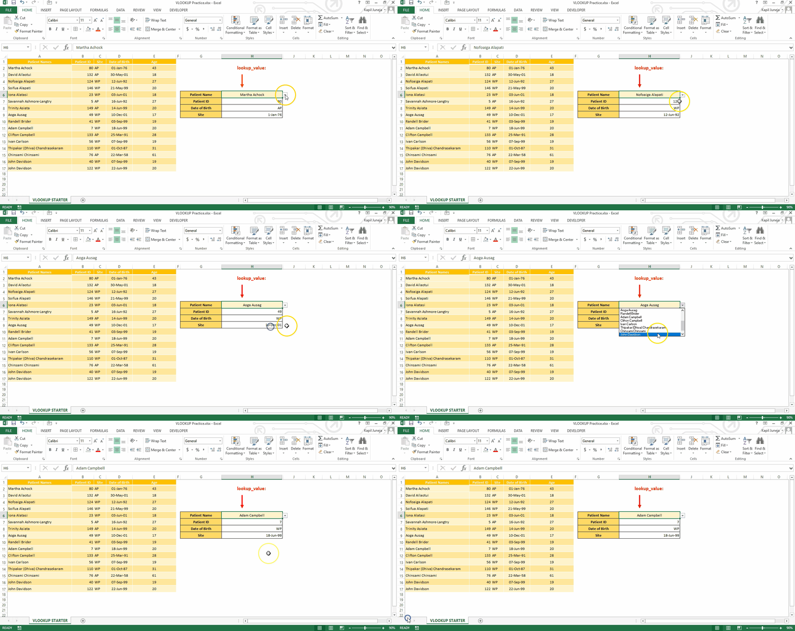
VLOOKUP is a vertical lookup which helps the user to extract the values from other columns (leftmost) basis on matching column string. Below is an image to explain you the same.
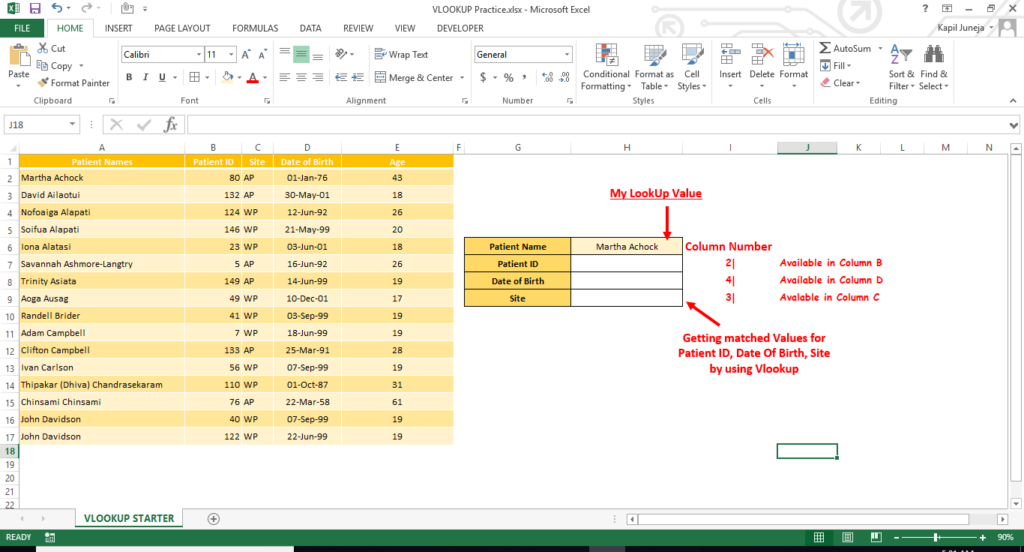
So in above example, we will get the Patient ID, Date of Birth, Site by using VLOOKUP Function for patient name mentioned in Cell H6
How to Write Excel VLOOKUP Formula?
Now while looking at above Formula, there are four parameters which are described as below:
lookup_value: this is a matching value which we will find in our database to locate the position and get respective values from different columns from the same position
table_array: this is our database where we will find our matching value and get the respective left most column value
col_index_num: this is a column position or column address from where we need the value depending on the matched string of different column
[range_lookup]: here will be instructing the excel whether to find approximate match for the given lookup value or to find exact match
Still Need Help in VLOOKUP Parameters: See below picture. Hope this helps 😊
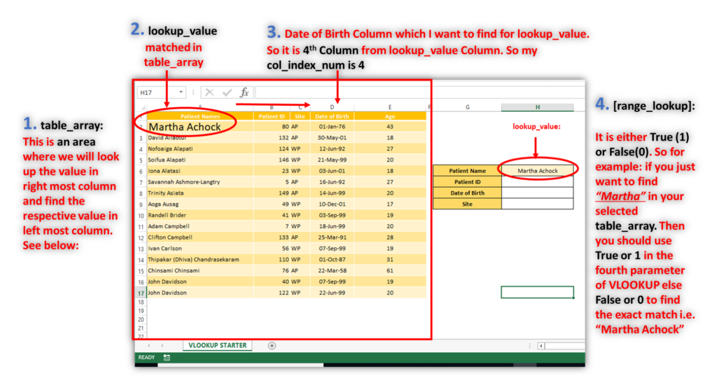
So here we have an example in Cell H6 “Martha Achock” and will get the Patient ID, Date of Birth, Site in H7,H8,H9 respectively. Below are the formulas which we need to write for getting these values:
Cell H7: “=VLOOKUP($H$6,$A$1:$E$17,2,0)”
Cell H8: “=VLOOKUP($H$6,$A$1:$E$17,3,0)”
Cell H9: “=VLOOKUP($H$6,$A$1:$E$17,4,0)”
This will get the respective VLOOKUP value for given Lookup value from the table_array.
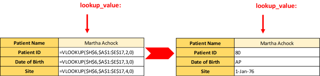
That’s how you can use VLOOKUP for standardizing big databases and linking the different excel files.
Points To Remember
- VLOOKUP finds the value in the left most column only
- Col_Index_Num is the position from where we want to extract the value
- Use Absolute range while copying or filling down the same formula from one cell to another cell
- [range_lookup): False or 0 is commonly used for the 4th Parameter in Vlookup. It helps to find exact match
Subscribe Our Blog to get more updates on Vlookup trick in Excel.






Really this is very nice article…and this is easy to understand..