Microsoft Excel “TODAY” function is used to get the current Date. It is very useful function and can be used in many ways. “TODAY Function” does not have any argument that makes this easy to apply and implement.
Date derived from TODAY function changes each time worksheet is refreshed/ edited/open/changed. So, ensure to Paste special values the formula output so that database is not changed. We will also discuss in below that how we can Paste special values.
“TODAY” function is very advantageous in many ways. It helps for the document where current Date details are required in more often. Applying current Date manually (one by one) to document is very difficult and “TODAY Function” helps to apply the function in large database at once and makes the work easy, saves time and increases efficiency.
“TODAY Function” is very useful and can be used in many situations. Like it can be used as follows:
– Document where Date stamps are required more often.
– Preparing time and motion study and day wise summary for employees
– Employees utilization or productivity, attendance tracker
– Or any other database where there is requirement of current Date stamps, “TODAY Function” can be used
=TODAY()
There are no arguments for “TODAY” function. Just apply the function and click “Enter”. It will show the current Date.
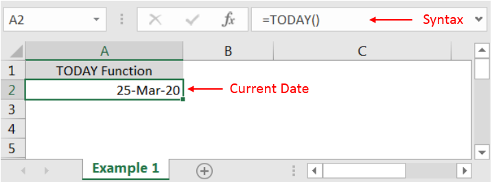
If output of the function is not as per the above (i.e. DATE), then we need to change the cell format. Follow below steps to change the format of the cell:
Step 1: Select the Cell or Data Range
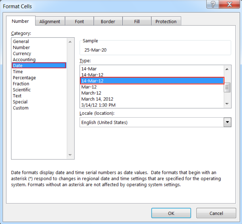
Step 2: Press Ctrl + 1 to open “Format Cells” option
Step 3: Select the option as per below i.e. Date -> 14-Mar-12
Step 4: Click to “OK”
This will change the format of the cell to desired format. We can change ANY of the Date or Time format as given in “Format Cell” option.
Values derived from TODAY function changes each time worksheet is refreshed/ edited/open/changed. So, ensure to Paste special values the formula output so that database is not changed.
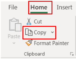
Below are the steps for paste special database to values:
– Select the data range -> Go to Menu Bar- > Click to Home-> Click to Copy
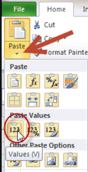
Then -> Go to Menu Bar- > Click to Home-> Click Paste Values
Hope you learnt this Function
Don’t forget to leave your valuable comments!
If you liked this article and want to learn more similar tricks, please Subscribe us.

Merge Cells in Excel Merge cells is to combine multiple cells into one cell which can further be used for giving title to the report or header to the column. It helps to create clean…

Watch: How to use SUMIF & SUMIFS Function in Excel? What is SUMIF Function? The SUMIF function in Excel adds up values in a range of cells that meet certain criteria. Click here to Read Full…

Watch: How to use COUNTIF & COUNTIFS Function in Excel? What is COUNTIF Function? In Excel, “COUNTIF” counts the number of cells within a range that meet a single specified criteria. Click here to Read…

MIN function is used to get the smallest number in range or list of values.MIN function has one required i.e. number1 and optional argument i.e. [number2]

This tutorial explains how the TRANSPOSE function works and shows you the right way to use it to switch data in Excel.
Everyone has different preferences, even for work habits. Some people like to arrange data in vertical columns, while others prefer horizontal rows. If you ever need to switch the direction of your data quickly, the TRANSPOSE function can help

The tutorial explains how to use the CHOOSE function in Excel, showing you the basics and some interesting examples. While CHOOSE might seem simple on its own, when you combine it with other functions, it can be powerful. Essentially, the CHOOSE function helps you pick a value from a list based on its position. The tutorial also covers some advanced ways to use CHOOSE that you might find very useful.