FIND function is used to locate the position of text, or character in an available string.
FIND Function has argument two required arguments i.e. find_text, within_text and one optional argument i.e. [start_num]. If no value is provided in [start_num] argument then function will take the Default value i.e. 1
=FIND(find_text, within_text, [start_num])
find_text argument, is used to give text, character or cell reference that is required to find
within_text argument, is used to give the cell reference from which text (i.e. find_text value ) to be searched
[start_num] is optional argument and is used to specify the character from which search should start. By default, the first character is 1, however if you want search should be started from 2nd find_text value then it should be position of 2nd find_text value and so on..
Here we have some examples, where:
– “Column A” has various strings,
– “Column B” shows the sample formula that is applied,
– “Column C” shows the output of the function and
– Explanation is provided in “Column D

– Output in Cell “C2” i.e. “6” is showing that the character “u” is available at “once upon” and “u” has 6th position.
– Output in Cell “C3” i.e. “13” is showing that the character “T” is available at “Tree” and has 13th position. Also note that character “t” is ignored in “there”
– Output in Cell “C4” i.e. “8” is showing that the character “t” is available at “tree” after ignoring character “t” at “that”.
– Find function is case sensitive, means it will only search “t” for text “the” and not with “The”. If you want to find value without case sensitive, then try “SEARCH” Function
– Find function will not work with Wild characters i.e. asterisk (*), question mark (?)
– Function should give output in “General” format, however if output is not as per the desired format then we need to change the cell format to “GENERAL”.
– If function parameters are not correctly applied in the function, then it will give output as “#VALUE!” (Error).
Don’t forget to leave your valuable comments!
If you liked this article and want to learn more similar tricks, please Subscribe us

Watch: How to use WEEKNUM Function in Excel? What is WEEKNUM Function? The WEEKNUM function in Excel returns the week number of a given date. It is a DATE and TIME function that can be…

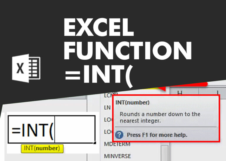
INT function is used to round down the numeric value to nearest integer. INT Function has one required argument i.e. number.

TRIM function is used to remove the additional spaces (i.e. spaces before/after/between the words) except for single space between words.

WEEKDAY function applies to a Date and returns the output for Day of the week. The output of the function varies from 0 to 7

The Article of DATEVALUE explains how to use Excel functions to change text into dates and numbers into dates. It also shows how to convert text strings into dates without using formulas. You’ll also learn…

This guide will show you quick and easy methods to find the number of days between dates in Excel.
Do you need to know how many days are between two dates? Maybe you want to find out the days between today and a date in the past or future, or just count the working days between two dates? Whatever you need, one of the examples below will help you find the solution