While working with Microsoft Excel, did you get a situation where you need to extract the characters from a string? I believe most of your answers are YES. In the said scenario “MID” function will help you to find the solution. We will be learning the Microsoft Excel “MID” in details, so stay with us and continue reading…
MID function is used for extracting the mid characters from the available string. The output of the function returns the extracted characters in new cell.
Function should give output in “General” format, however if output is not as per the desired format then we need to change the cell format to “GENERAL”.
MID Function has argument three arguments i.e. text, start_num and num_chars where we need to give the cell references and parameters. We can give the parameters as per the requirement by following the “ , “ (i.e. Comma) as separator.
If parameters are not separated by “ , “ (i.e. Comma) or quotation mark is/are missing or any other function error then it will give output as “#VALUE!” (Error). So always ensure that function parameters are used to get the appropriate results/output.
=MID(text,start_num,num_chars)
Excel MID Function has three compulsory parameters, i.e, text, start_num, num_chars
The MID function in Excel is very simple and easy to use. Let us understand the working of the MID function in Excel by some MID formula example.
We will be following MID function as follows:
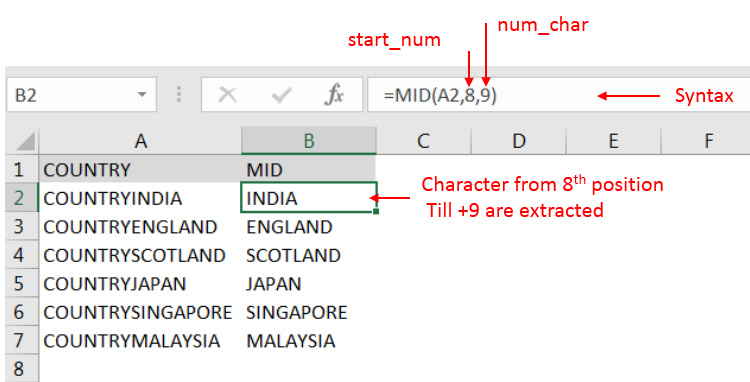
– “text argument”: “A2” is the cell reference from which characters should be extract
– “start_num argument”: “8” is the 8th character from string should be extracted
– “num_char argument”: “9” is the total number of characters from the string should be extracted starting from 8th character

Explanation: we can see ignored “COUNTRY” has total 7 character that is why character 8th position is mentioned in “start_num argument”. Also, total 9 characters are required after 8th that is why “9” is mentioned in “num_char argument” i.e. till 8+9 = 17 characters
Hope you learnt this Function,
Don’t forget to leave your valuable comments!

Count Non Blank Cells in Excel helps you to ignore blank ones and focus only on cells with values that matter to you. Some cells in an Excel worksheet may look blank but aren’t actually…

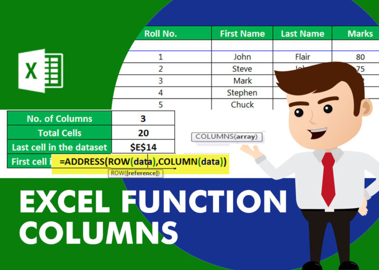
COLUMNS function is used to get the total count of columns in an array or in cells range for excel worksheet.

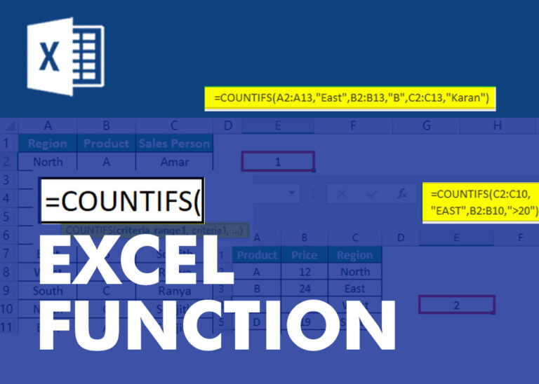
COUNTIFS function is used to get the total count for number of times the various criteria across ranges are met.

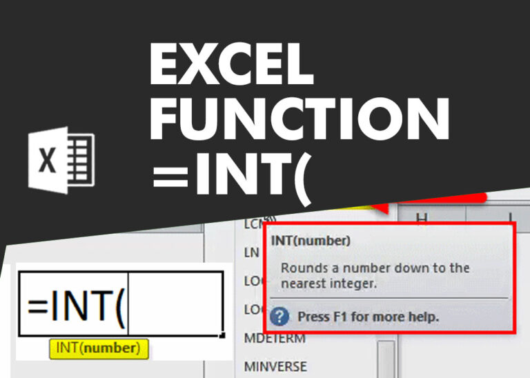
INT function is used to round down the numeric value to nearest integer. INT Function has one required argument i.e. number.

The tutorial demonstrates how to find a date any number of days before or after today, counting either all days or only business days.

Watch: How to use VLOOKUP Function in Excel? What is VLOOKUP Function? The VLOOKUP function in Excel searches for a value in a table and returns a corresponding value from another column in the same row…