COUNTIFS function is used to get the total count for number of times the various criteria across ranges are met.
COUNTIFS Function has one required arguments i.e. criteria_range1, criteria1 and Optional arguments i.e. [criteria_range2, criteria2]…
We can place multiple criteria or conditions in function by separating them with comma ( , )
=COUNTIFS(criteria_range1, criteria1, [criteria_range2, criteria2]…)
criteria_range1 argument is used to give the range in which criteria1 needs to find
criteria1 argument is used to give criteria for count. We can give value (example “A”, >10, 50) or cell reference# (example: F2) in this argument
[criteria_range2] optional argument is used to give the ANOTHER range in which criteria2 needs to find
[criteria2] optional argument is used to give criteria2 for count. Value or cell reference# can be given.
Kindly note, we can add multiple criteria in the function by separating them with Comma ( , )
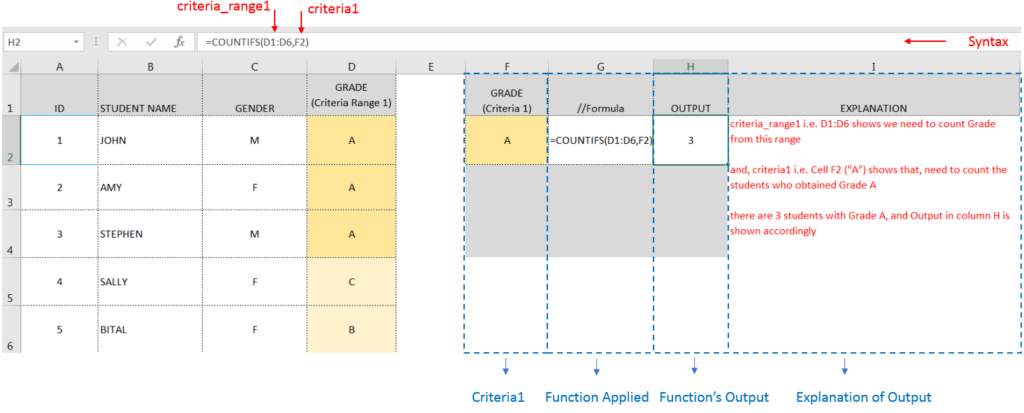
Here, we want to get the count of students who obtained Grade A:
We will be using COUNTIFS function as follows:
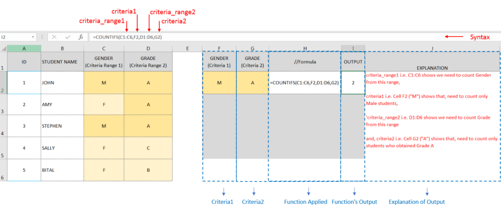
Here, we want to get the count of Male Students (criteria1) who have obtained Grade A (criteria2):
We will be using COUNTIFS function as follows:
Hope you learnt this Function,
Don’t forget to leave your valuable comments!
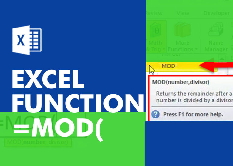
MOD function is used to get the remainder of number that is divided by divisor. MOD Function has two required arguments i.e. number and divisor.

LARGE function is used to get the Largest k-th value from the range.
LARGE Function has two required arguments i.e. array, and k
VBA Code to Count Color Cells With Conditional Formatting Have you ever got into situation in office where you need to count the cells with specific color in conditional formatted Excel sheet? If yes then…

How to use Excel Function PROPER? PROPER function is used for changing the format of any text or string to PROPER or SENTENCE Case. PROPER Function has argument only one argument i.e. text, which makes the function…
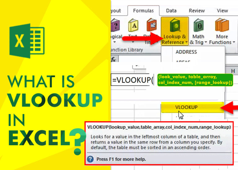
An ultimate guide for basic user to understand Excel Vlookup function. VLOOKUP is a vertical lookup which helps the user to extract the values from other columns (leftmost) basis on matching column string.

SEARCH function is used to find “position of character or text” in an available cell and this function is NOT case sensitive.