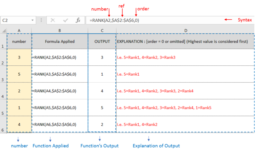
RANK function performs the Ranking in a range or list of numbers. Function returns the rank position and can assigned as Highest or Lowest value as 1st rank as per order argument.
Syntax:
=RANK(number,ref,[order])
number argument is used to give number value for which ranking is required
ref argument is used to give range or list of values from which rank to measure
[order] is optional argument and Value 0 or 1 can be given as per below requirements:
[order] = 0 or omitted: Highest value will be Ranked as 1st position (example: Value 5=Rank1, 4=Rank2, 3=Rank3, 2=Rank4, 1=Rank5 and so on)
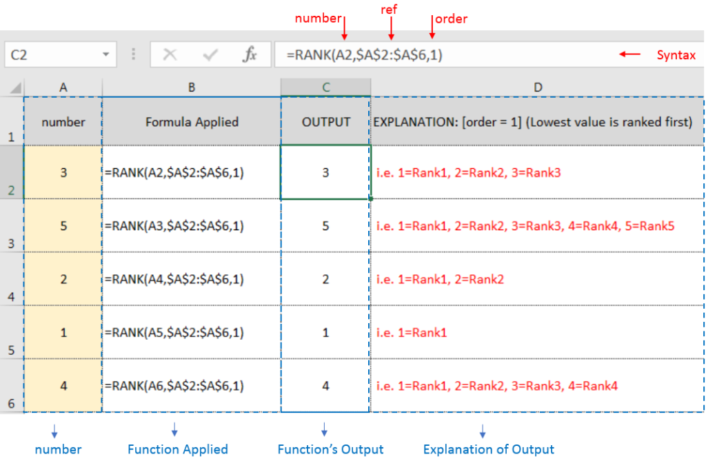
[order] = 1: Lowest value will be Ranked as 1st position (example: Value 1=Rank1, 2=Rank2, 3=Rank3, 4=Rank4, 5=Rank5 and so on)
Example 2: RANK function with [order = 1] (Lowest value is ranked first)
Example 3: RANK function with [order = 1] (Lowest value is ranked first) with Repeat values
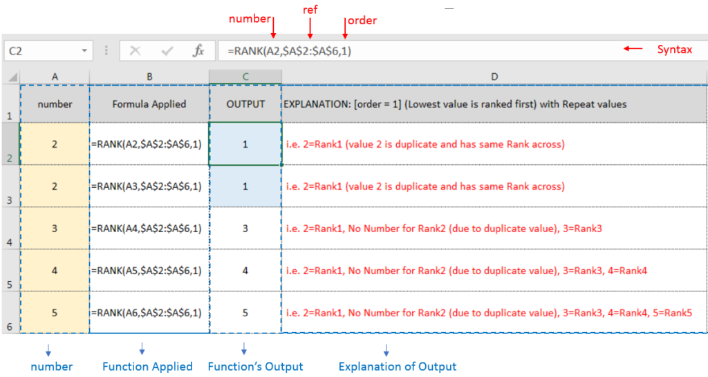
If list of values or ref argument has duplicate values, ranking for those values will be same across
Hope you learnt this Function,
Don’t forget to leave your valuable comments!
If you liked this article and want to learn more similar tricks, please Subscribe us or follow us on Social Media by clicking below buttons:

Conditional Formatting helps to easily identify the usual and unusual numbers/ conditions, creating interactive visualization by means of Highlight Cells by Rules, Top/Bottom Rules, Data Bars, Color Scales and Icon Sets.
Excel Function ISERROR Microsoft Excel “ISERROR Function” is a Logical Function and it is used to check if cell contains any “ERROR”. “ISERROR Function” is used as a test to validate if cell contains any…

Create Dynamic Data Validation List When I started my career in working with excel dashboards, I always used to face most common challenge in “Data Validation” technique where I want a smart data validation to avoid all…

Scroll Lock in Excel can make scrolling, selecting cells, checking formulas, entering data, and recording macros harder. So, you might need to turn it off to work normally. In this article, we’ll show you how…
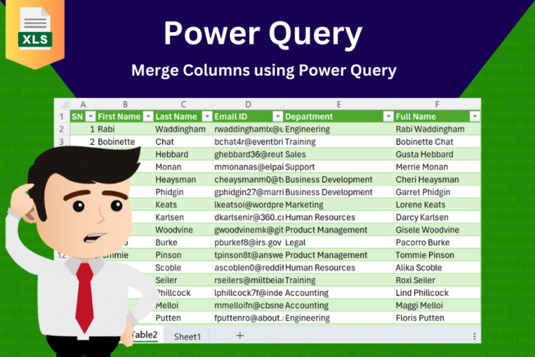
In this tutorial, learn how to merge columns using Power Query. Follow this step-by-step guide to convert data into a table, merge columns seamlessly, and customize separators. Whether you’re a beginner or an advanced user, this tutorial will enhance your data manipulation skills and streamline your workflow. Master Power Query and optimize your data management processes effortlessly.

This tutorial explains what an Excel name is and shows you how to define a name for a cell, range, constant, or formula. You’ll also learn how to edit, filter, and delete defined names in Excel.
Excel names are a bit of a paradox: they’re one of the most useful features, but many people find them unnecessary or too technical. That’s because few users truly understand what Excel names can do. This tutorial will not only teach you how to create a named range in Excel but also show you how this feature can make your formulas easier to write, read, and reuse.