Are you struggling with merging columns in Power Query? Don’t worry! In this comprehensive guide, we’ll walk you through the process step by step so you can easily merge columns in Power Query.
Step 1: Convert Data into a Table
To begin, you need to convert your data into a table. There are two simple methods to do this:
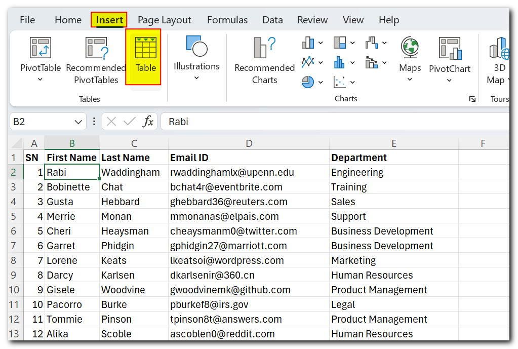
Go to the “Insert” tab, select the range containing your data, and convert it into a table.
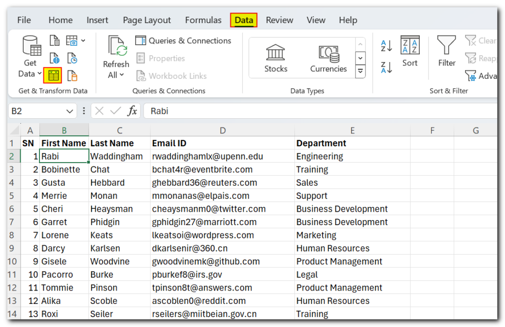
Alternatively, navigate to the “Data” tab, choose “From Table/Range,” and Power Query will automatically convert your data into a table.
Step 2: Access Power Query
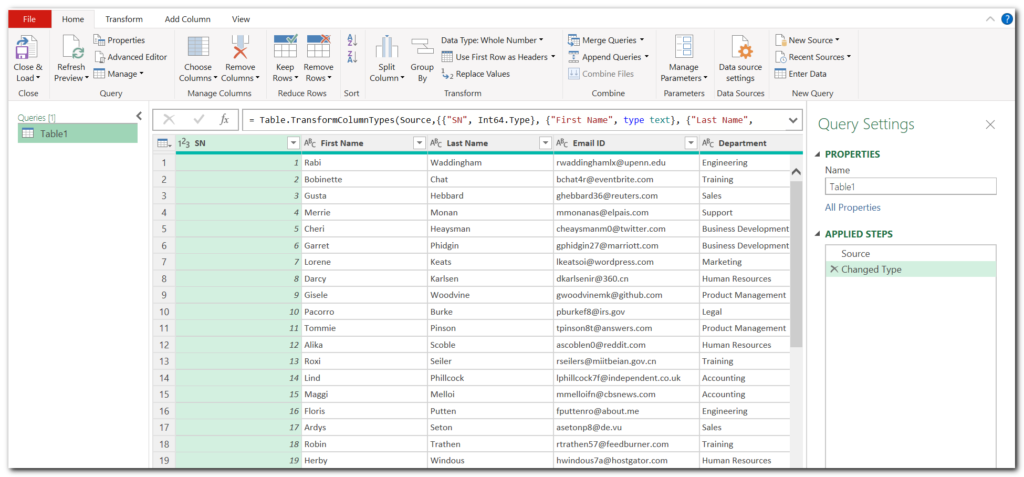
Once your data is in table format, Power Query will open automatically. Here, you’ll see all your columns displayed neatly.
Step 3: Merge Columns
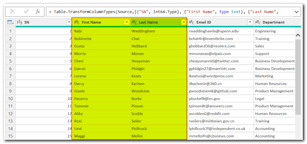
Now, let’s merge the columns. Suppose you want to merge the “First Name” and “Last Name” columns to create a “Full Name” column. Select both the “First Name” and “Last Name” columns (use shift key to select multiple columns).
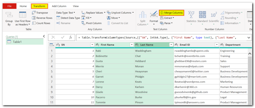
Click on the “Merge Columns” option under Transform menu.
Step 4: Configure Merge Settings
A popup window will appear with merge options.

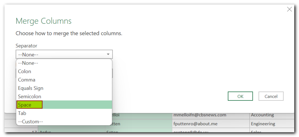
You can choose a separator to distinguish between merged values. Typically, a space works well for creating full names. Select the space character as the separator.
Name the new column “Full Name” in the designated field.
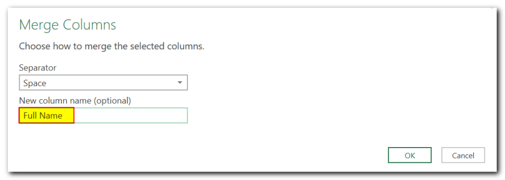
Click “OK” to proceed.

Step 5: Review and Load Data
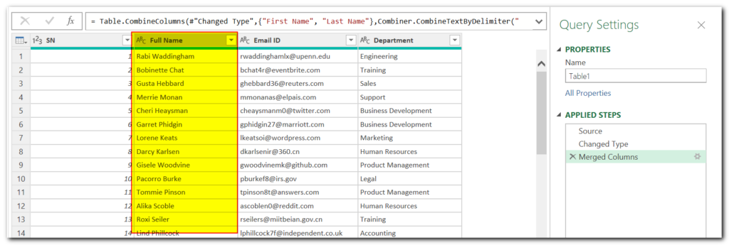
Once merged, the “Full Name” column will appear, combining the first and last names seamlessly.
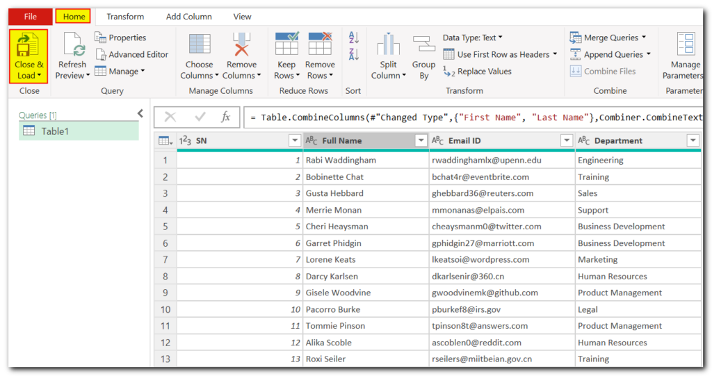
Click on “Home” and choose “Close and Load.”
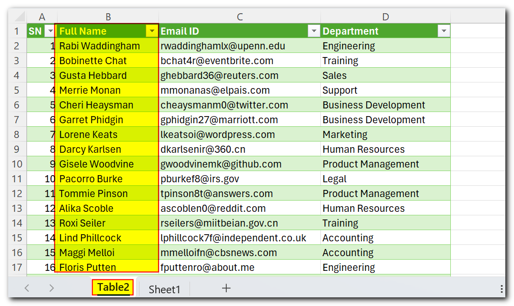
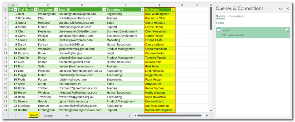
The merged data will be loaded into a new sheet, ready for further analysis or presentation.
Alternate Method to keep Original Columns
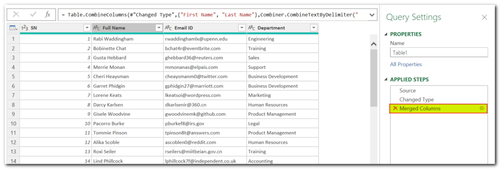
Step 1: Delete the recently added merged columns step.
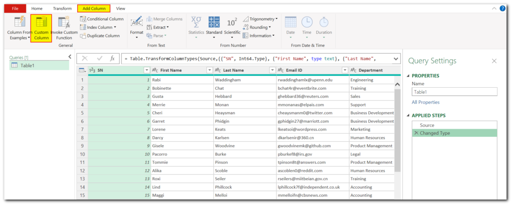
Step 2: Under “Add Column” menu, click on “Custom Column”
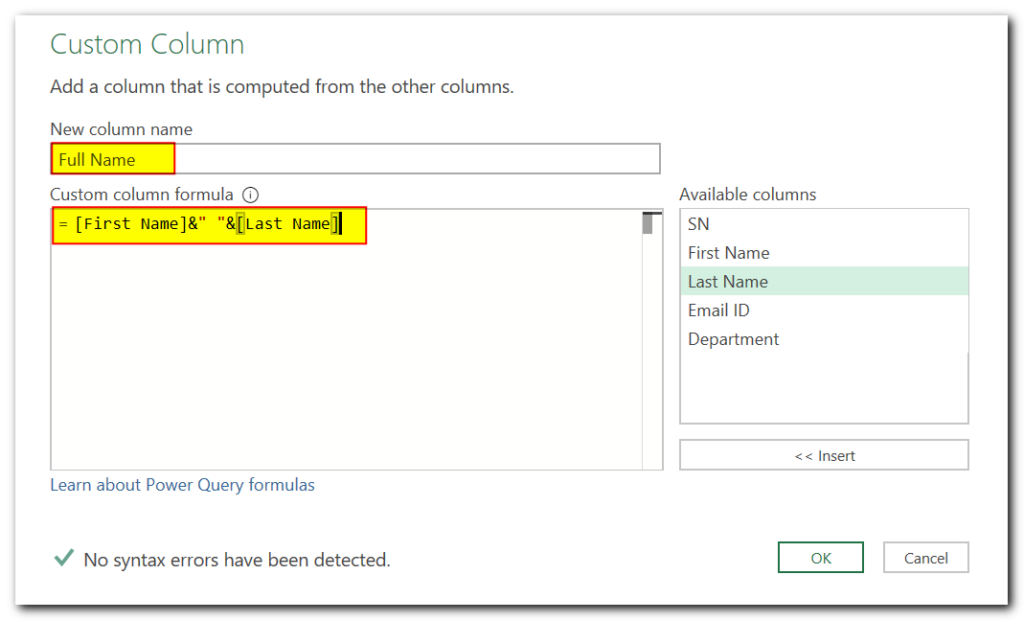
Step 3: Write the new column name as “Full Name” and mention the formula as “=[First Name]&” “&[Last Name]”.
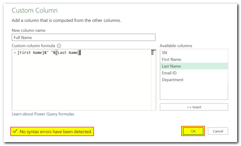
Step 4: Make sure there is no syntax error in your formula. Once done, click on Ok
Step 5: You will notice this time a new column “Full Name” is added at the end.

Step 6: Once done with all query changes, click on “Home” and choose “Close and Load.”
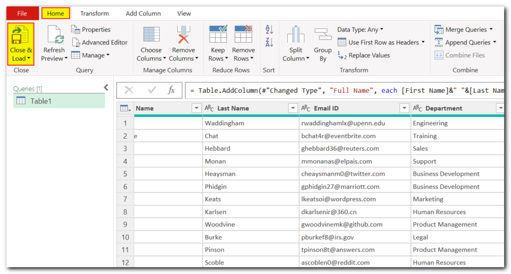
Step 7: Your newly merged data will be loaded into a new sheet, ready for further analysis or presentation.
That’s it! You’ve successfully merged columns using Power Query. Whether you prefer the built-in merge option or custom formulas, Power Query offers versatile solutions to meet your data manipulation needs.
Thank you, we hope this guide has been helpful in enhancing your data management skills with Power Query. Stay tuned for more insightful tutorials!


