While working with Microsoft Excel, did you get a situation where you need to extract the Right-side characters from a string? I believe most of your answers are YES. In the said scenario “RIGHT” function will help you to find the solution. We will be learning the Microsoft Excel “RIGHT” in detail, so stay with us and continue reading…
Function should give output in “General” format, however if output is not as per the desired format then we need to change the cell format to “GENERAL”.
RIGHT Function has argument two arguments i.e. text and num_chars where we need to give the cell references and parameters (i.e. count of characters required from right side in number format), we can give the parameters as per the requirement by following the “ , “ (i.e. Comma) as separator.
If parameters are not separated by “ , “ (i.e. Comma) or quotation mark is/are missing or any other function error then it will give output as “#VALUE!” (Error). So always ensure that function parameters are used to get the appropriate results/output.
RIGHT function is very advantageous in many ways. It helps for the document where extracting of characters from an available string is required. Extracting characters from an available string manually (one by one) in a report is very difficult and RIGHT Function helps to apply the function in large database at once and makes the work easy, saves time and increases efficiency.
=RIGHT(text,num_chars)
text argument, is used to give the cell reference from which characters should be extracted
num_chars argument, is used to give the numeric value of total count of characters you want to extract from right side of a string
– Spaces available in a string is counted as characters
– Currency symbols are not counted as characters and will be ignored by the function
– If “num_chars argument” field is blank, it will be counted as 1 (by default) and 1st character of the string will return as output
– “num_chars argument” should not be a negative value otherwise function output will return to “#VALUE!” (Error)
– If value in “num_chars argument” is greater than the total count of characters in a string, then function’s output will return the complete string.
– Function should give output in “General” format, however if output is not as per the desired format then we need to change the cell format to “GENERAL”.
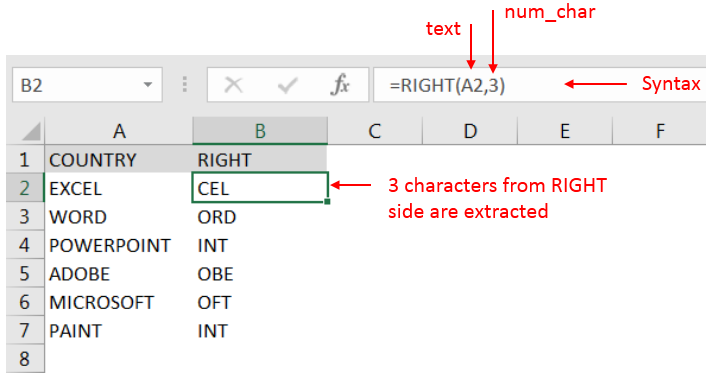
Here, we have a column with Application names and there is requirement of extraction of last Right three character.
We will be following RIGHT function as follows:
“text argument”: “A2” is the cell reference from which characters should be extract
“num_char argument”: “3” is the total number of count of characters required from right side

Explanation: We can see in cell “A2” has string as “EXCEL” and right function extracted total 3 characters from a sting and “CEL” is returned as output in cell “B2”
Hope you learnt this Function!
Don’t forget to leave your valuable comments!
If you are liking our articles and want to learn more similar tricks, please Subscribe us or follow us on Social Media by clicking below buttons.

This tutorial introduces XLOOKUP, a new function in Excel for both vertical and horizontal lookups. Tasks that used to feel super complicated, like left-side lookups, finding the last match, or using VLOOKUP with multiple criteria, are now much easier with XLOOKUP.
Before, you had to choose between VLOOKUP for vertical lookups, HLOOKUP for horizontal ones, or more complex options like INDEX MATCH or Power Query. But now, you don’t have to pick anymore. XLOOKUP can handle all those tasks in one simple function.

Microsoft Excel is a useful tool for analyzing data and conducting statistical research. The program includes numerous functions for performing various statistical calculations. One of the essential measures Excel supports is the weighted average.

SUMIFS function is used to get the “total sum” of values for matching criteria across range. SUMIFS Function has required and optional arguments

Watch: How to use MODE & MODEIF Function in Excel? What is MODE Function? In Excel, the “MODE” function is a statistical tool that identifies and returns the most frequently occurring value within a set…

Understand how to find median in Excel with simple steps. Understanding the middle value in a set of numbers, known as the median, is important in the data industry. Professionals often use Microsoft Excel to calculate this. Excel’s MEDIAN function helps quickly find this value from long lists of numbers. This saves time and allows for further calculations using the median value. In this article, we explain what the MEDIAN function in Excel does, why it’s useful, and two methods to find the median in your data.

Excel Function DATE When you work with dates in Excel, the DATE function is crucial to understand. The reason is that some other Excel functions may not always recognize dates when they are entered as…