Excel Function SUMIFS is used to get the “total sum” of values for matching criteria across range.
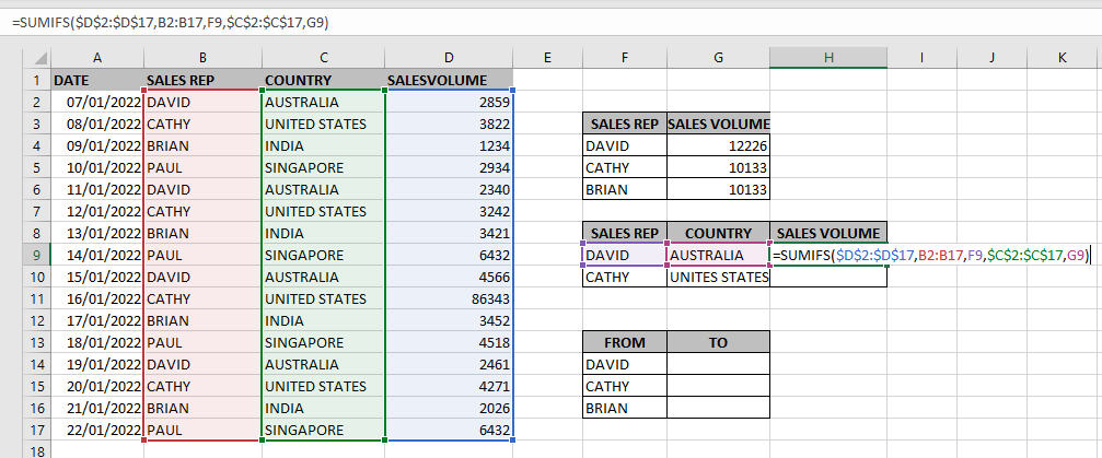
SUMIFS Function is used to get total sum with more than one criteria. It has required arguments i.e. sum_range, criteria_range1, criteria1 and Optional arguments i.e. [criteria_range2, criteria2]… We can place add more than one range to include multiple criteria or conditions.
SUMIFS function is used to get the “total sum” of values for matching criteria across range.
SUMIFS Function has required arguments i.e. sum_range, criteria_range1, criteria1 and Optional arguments i.e. [criteria_range2, criteria2]… We can place add more than one range to include multiple criteria or conditions.
The syntax is as follows:
SUMIF(range, criteria, [sum_range])
sum_range argument is used to give cell range; those are to be added together as per the criteria mentioned below
criteria_range1 argument is used to give the range in which criteria1 needs to find
criteria1 argument is used to give criteria for sum. We can give value (example “A”, >10, 50) or cell reference# (example: E2) in this argument
[criteria_range2] optional argument is used to give the ANOTHER range in which criteria2 needs to find
[criteria2] optional argument is used to give criteria2 for sum. Value or cell reference# can be given.
Kindly note, we can add multiple criteria in the function by separating them with Comma (,)
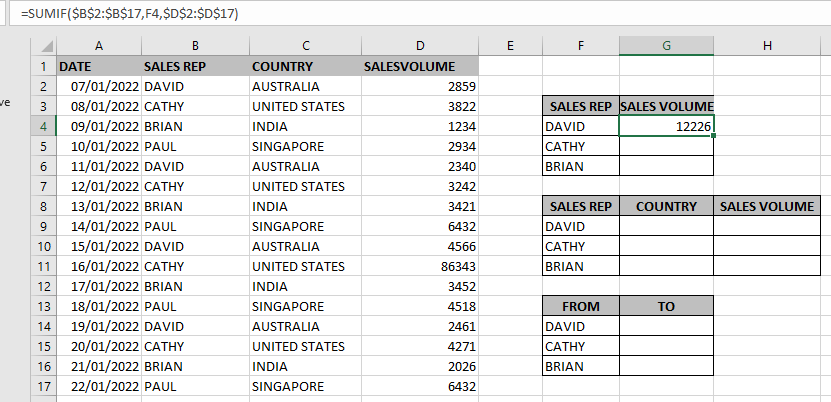
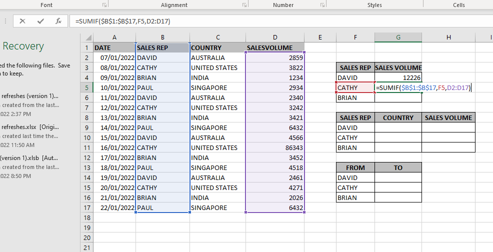
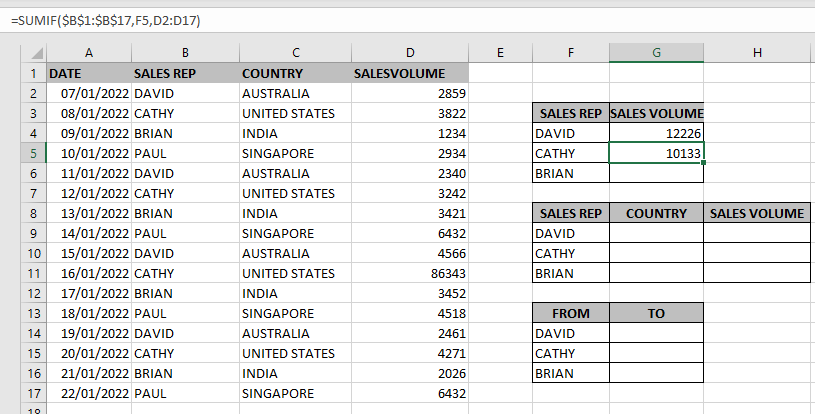
We will be using SUMIF function as follows:
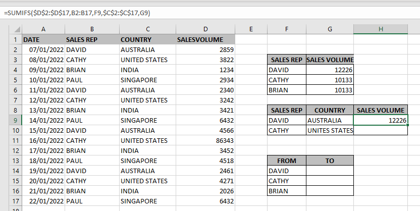
Hope you learnt this Function,
Don’t forget to leave your valuable comments!
If you liked this article and want to learn more similar tricks, please Subscribe us.

LEN function is used for counting number of characters in available string. The output of the function returns the count in new cell.

Microsoft Excel “DAY, MONTH, YEAR Functions” are date related functions helps to extract the Day, Month or Year from a Date.
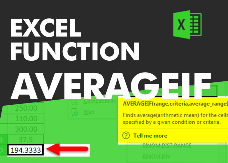
AVERAGEIFS function is used to get the “average” of values for matching criteria across range. Average = Sum of all values / number of items.

SUBSTITUTE function is used to substitute the existing old text to new text.
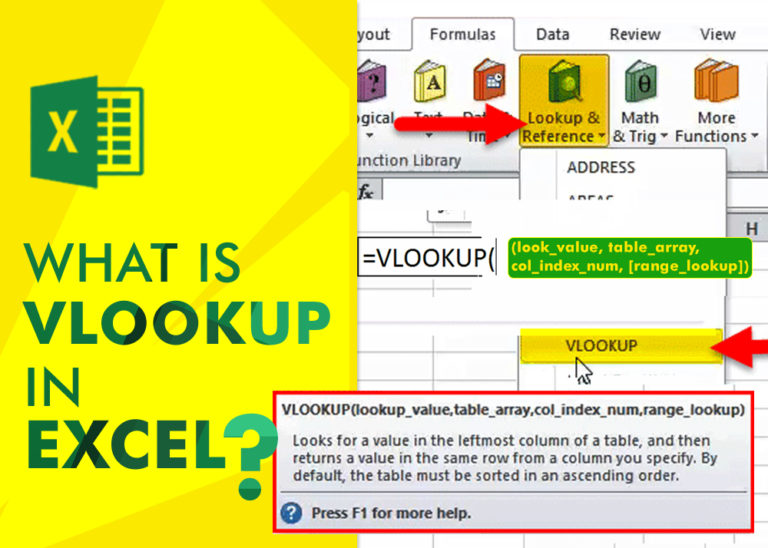
An ultimate guide for basic user to understand Excel Vlookup function. VLOOKUP is a vertical lookup which helps the user to extract the values from other columns (leftmost) basis on matching column string.

WEEKDAY function applies to a Date and returns the output for Day of the week. The output of the function varies from 0 to 7