=TEXT(value,format_text)
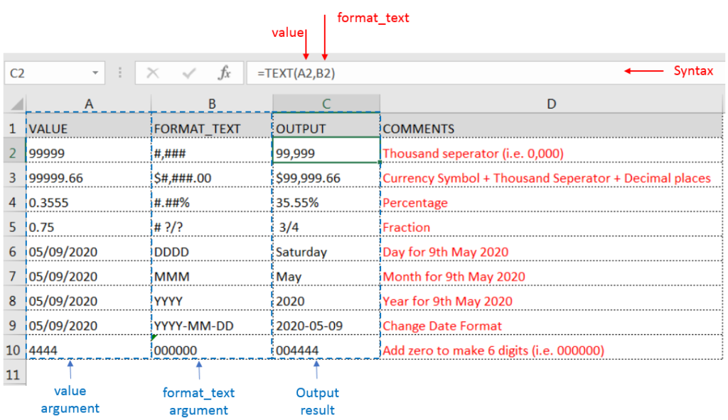
value argument [Required] is used to give the text or cell reference for which formatting is to be changed
format_text [Required], is used to give the formatting code as per the requirement
Here we have some examples, where “Column A” has various values, “Column B” represents format_text and “Column C” shows the output of the function.
We will be using TEXT function as follows:

– Format of cell can also be changed by following CTRL+1 (or MAC Command button +1) and select the desired format/appearance
– If cell reference is not correctly provided in the function, then it will give output as an error
– Function should give output in “General” format, however if output is not as per the desired format then we need to change the cell format to “GENERAL”
Hope you learnt this Function,
Don’t forget to leave your valuable comments!
If you liked this article and want to learn more similar tricks, please Subscribe us or follow us on Social Media by clicking below buttons:

“NETWORKDAYS” function is very helpful feature in the Microsoft excel to calculate the working days from a particular period excluding “Saturday and Sundays”. NETWORKDAYS function subtract the Start Day from the End Date provided.

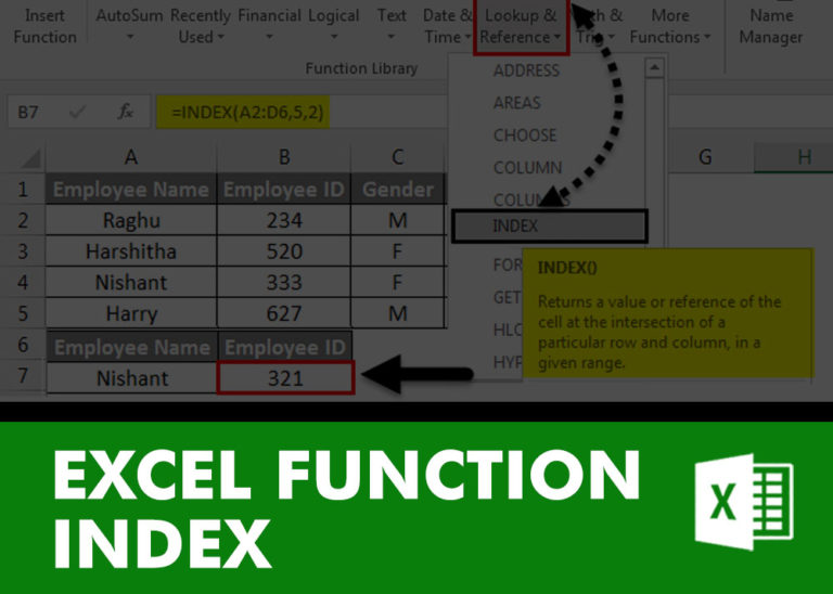
INDEX function is used to get the value from a cell range or table, function returns the value from a table where row and column intersect with each other.

Watch: How to use WEEKNUM Function in Excel? What is WEEKNUM Function? The WEEKNUM function in Excel returns the week number of a given date. It is a DATE and TIME function that can be…

This tutorial shows you how to change the row colors in Excel to automatically highlight every other row or every nth row or column in your worksheets. You will also learn how to use Excel’s banded rows and columns and find some helpful formulas to shade rows based on value changes.
Using alternating colors for rows in Excel is a common way to make data easier to read. While it’s simple to manually highlight rows in a small table, it can be very time-consuming in larger tables. A better approach is to automatically alternate the colors of rows or columns, and this article will show you how to do it quickly

Watch: How to use VLOOKUP Function in Excel? What is VLOOKUP Function? The VLOOKUP function in Excel searches for a value in a table and returns a corresponding value from another column in the same row…

MID function is used for extracting the mid characters from the available string. The output of the function returns the extracted characters in new cell.