WEEKNUM function helps to calculate the week number of the given date in a year. It considers 1st January as first week by default and through the output for the given input date.
=Weeknum(serial_number,[return_type])
WEEKNUM function helps to calculate the week number of the given date in a year. It considers 1st January as first week by default and through the output for the given input date.
=Weeknum(serial_number,[return_type])
The WEEKNUM uses the following arguments: Serial_number (required argument) – This is an Excel date for which we want to return the week number. When entering the argument, we should enter the date using the DATE function or as a result of other formulas or functions.
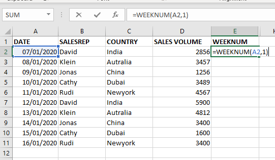
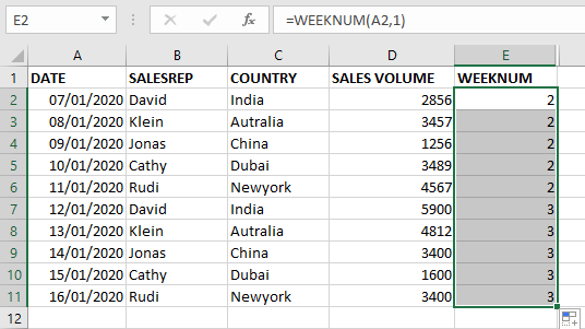
To find the WEEKNUM of the year we use the formula =WEEKNUM(A2,1).
In the WEEKNUM formula select the first argument as date comma now select first day of week it depends every company has different first day of week here i am selecting sunday .
As shown in below image when you apply formula the result is 2 and when we copy formula in column the result is shown in 2nd image.


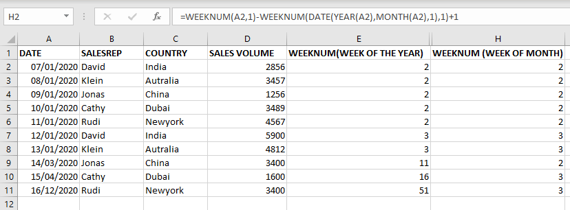
To get week of the month using the same WEEKNUM Formula.
Calculating the week of the year minus the week of the year of first of the same month.
FORMULA=WEEKNUM(A2,1)-WEEKNUM(DATE(YEAR(A2),MONTH(A2),1),1)+1


The ROMAN function in Excel converts numbers into Roman numerals. It’s useful when you need to display numbers in the Roman numeral format, such as for dates, titles, or other specific purposes. The function allows you to choose how “traditional” or simplified the Roman numeral should be. To use the ROMAN function, you just need to enter the number you want to convert, and Excel will do the rest

REPT function is used to repeat the text or cell reference to multiple times

Microsoft Excel is a useful tool for analyzing data and conducting statistical research. The program includes numerous functions for performing various statistical calculations. One of the essential measures Excel supports is the weighted average.

This tutorial explains how the TRANSPOSE function works and shows you the right way to use it to switch data in Excel.
Everyone has different preferences, even for work habits. Some people like to arrange data in vertical columns, while others prefer horizontal rows. If you ever need to switch the direction of your data quickly, the TRANSPOSE function can help

This tutorial introduces XLOOKUP, a new function in Excel for both vertical and horizontal lookups. Tasks that used to feel super complicated, like left-side lookups, finding the last match, or using VLOOKUP with multiple criteria, are now much easier with XLOOKUP.
Before, you had to choose between VLOOKUP for vertical lookups, HLOOKUP for horizontal ones, or more complex options like INDEX MATCH or Power Query. But now, you don’t have to pick anymore. XLOOKUP can handle all those tasks in one simple function.

FIND function is used to find the position of text, or character in an available string.