FIND function is used to locate the position of text, or character in an available string.
FIND Function has argument two required arguments i.e. find_text, within_text and one optional argument i.e. [start_num]. If no value is provided in [start_num] argument then function will take the Default value i.e. 1
=FIND(find_text, within_text, [start_num])
find_text argument, is used to give text, character or cell reference that is required to find
within_text argument, is used to give the cell reference from which text (i.e. find_text value ) to be searched
[start_num] is optional argument and is used to specify the character from which search should start. By default, the first character is 1, however if you want search should be started from 2nd find_text value then it should be position of 2nd find_text value and so on..
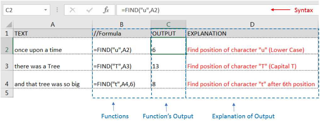
Here we have some examples, where:
– “Column A” has various strings,
– “Column B” shows the sample formula that is applied,
– “Column C” shows the output of the function and
– Explanation is provided in “Column D
– Output in Cell “C2” i.e. “6” is showing that the character “u” is available at “once upon” and “u” has 6th position.
– Output in Cell “C3” i.e. “13” is showing that the character “T” is available at “Tree” and has 13th position. Also note that character “t” is ignored in “there”
– Output in Cell “C4” i.e. “8” is showing that the character “t” is available at “tree” after ignoring character “t” at “that”.
– Find function is case sensitive, means it will only search “t” for text “the” and not with “The”. If you want to find value without case sensitive, then try “SEARCH” Function
– Find function will not work with Wild characters i.e. asterisk (*), question mark (?)
– Function should give output in “General” format, however if output is not as per the desired format then we need to change the cell format to “GENERAL”.
– If function parameters are not correctly applied in the function, then it will give output as “#VALUE!” (Error).
Don’t forget to leave your valuable comments!
If you liked this article and want to learn more similar tricks, please Subscribe us

WEEKDAY function applies to a Date and returns the output for Day of the week. The output of the function varies from 0 to 7

INDIRECT function is used to convert the text/string into cell reference. Function provides output as the value of that cell reference.

CONCATENATE function is used for combining two or more Microsoft Excel strings into one. The output of the function returns as a combined string in new cell.

Excel Function ISERROR Microsoft Excel “ISERROR Function” is a Logical Function and it is used to check if cell contains any “ERROR”. “ISERROR Function” is used as a test to validate if cell contains any…
COLUMNS function is used to get the total count of columns in an array or in cells range for excel worksheet.

“NETWORKDAYS” function is very helpful feature in the Microsoft excel to calculate the working days from a particular period excluding “Saturday and Sundays”. NETWORKDAYS function subtract the Start Day from the End Date provided.