Introduction
Welcome to this comprehensive guide on using Power Query in Excel to split data efficiently. In this tutorial, we’ll walk you through the step-by-step process of splitting columns, specifically focusing on splitting the name column into first name and last name and splitting the employee ID column based on a predefined pattern.
Step 1: Converting Data to a Table
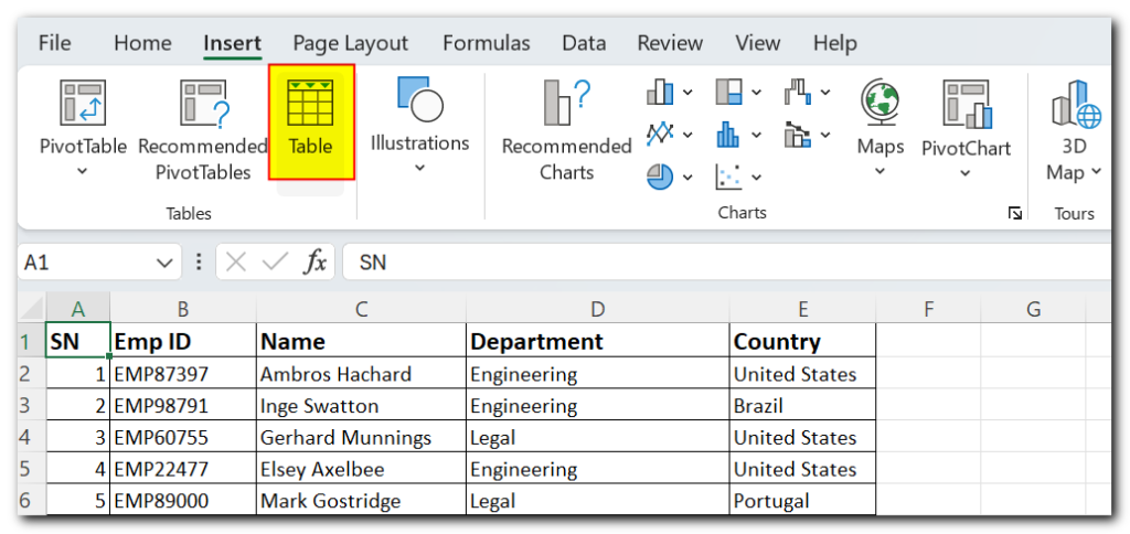
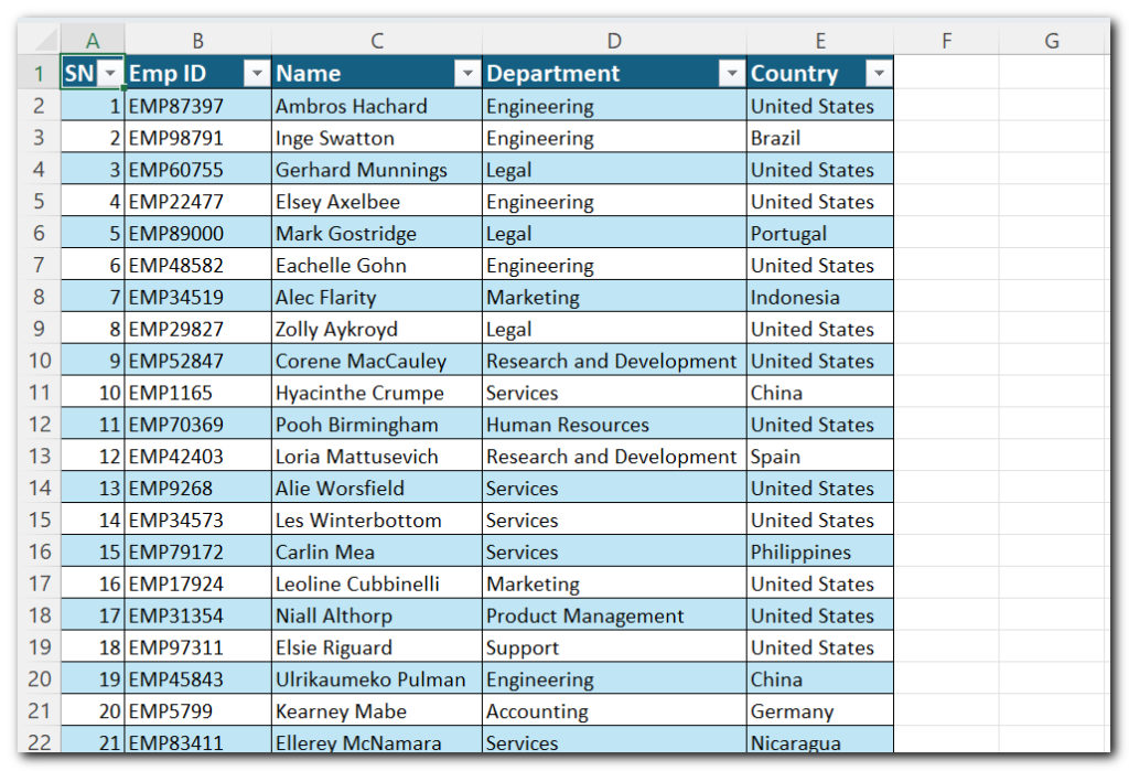
Begin by converting your data into a table. In Excel, navigate to the “Insert” tab and select “Table” to convert the range into a structured table format, which facilitates easier data manipulation.
Sample Data:
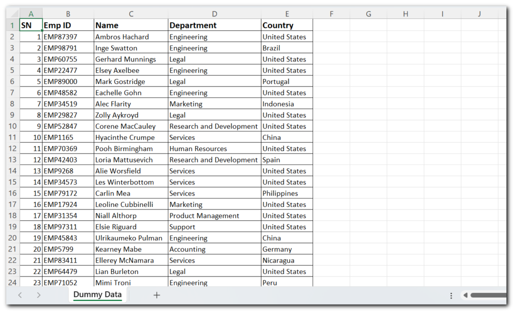
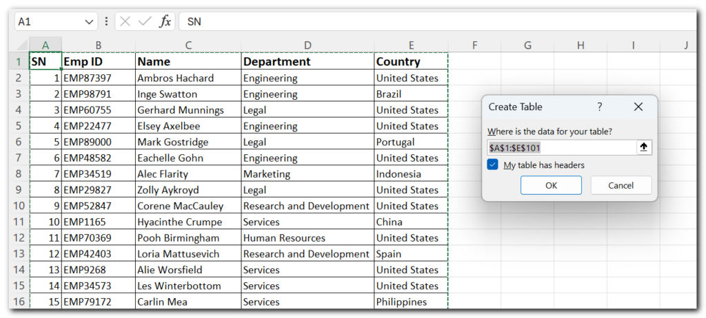
Converted Table:
Step 2: Accessing Power Query
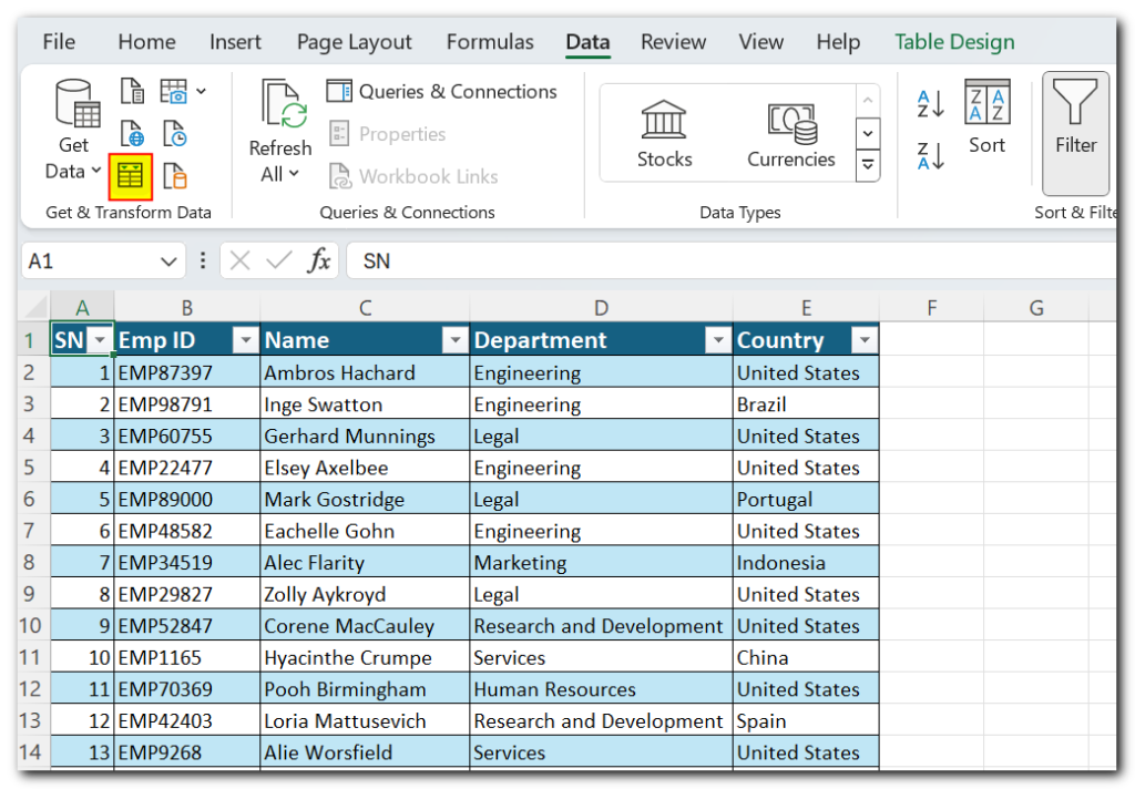
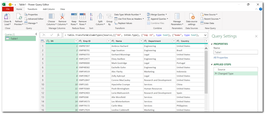
Once your data is in table format, head to the “Data” tab and click on “From Table/Range.” This action will open the Power Query Editor, providing you with powerful tools for data transformation.
Step 3: Splitting the Name Column
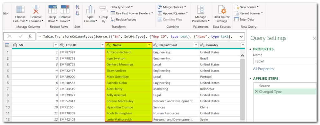
Locate the column containing the names in the Power Query Editor. Click on the column header and select “Split Column.” Choose the “Delimiter” option and specify a space as the delimiter. Ensure to select the advanced option “Split into Columns” to divide the name into separate columns for first name and last name.
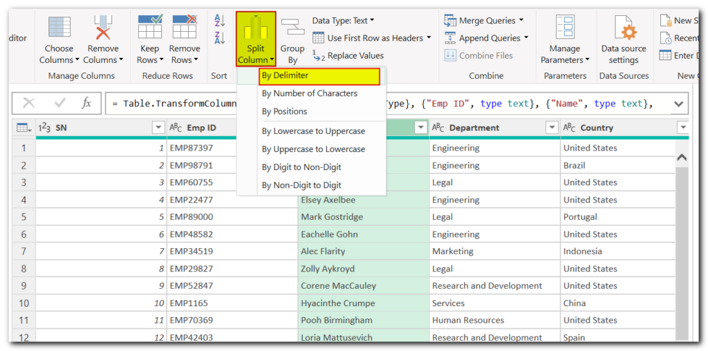
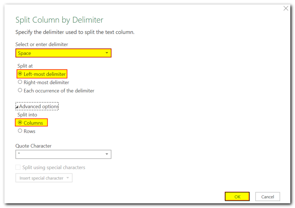
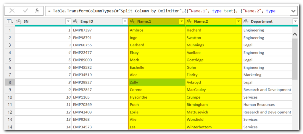
Step 4: Splitting the Employee ID Column
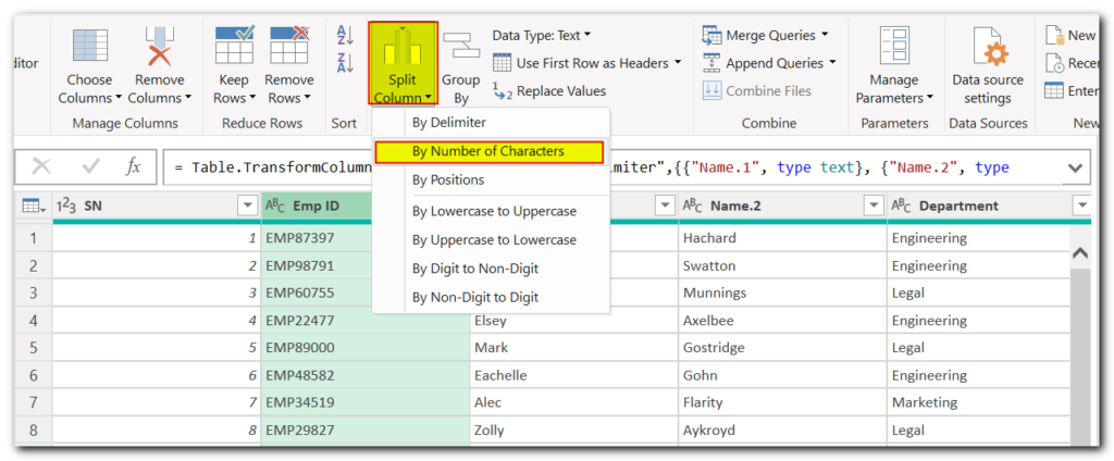
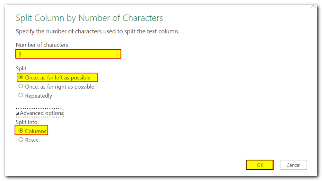
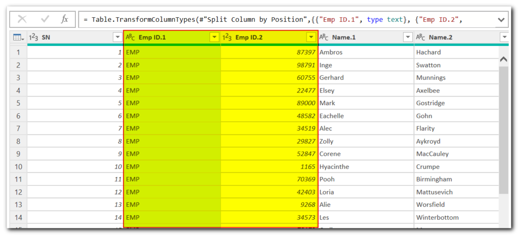
Identify the pattern in the employee ID column, such as a prefix followed by numeric values. For example, “EMP” followed by digits. Click on the column header, choose “Split Column,” and select “By Number of Characters.” Specify the number of characters to split after, typically the length of the prefix, to separate the prefix from the numeric values.
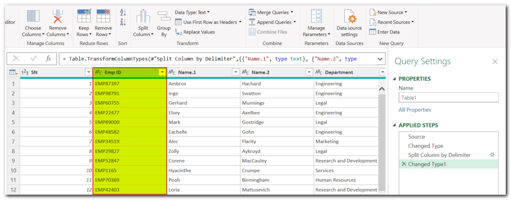
Step 5: Refining the Data
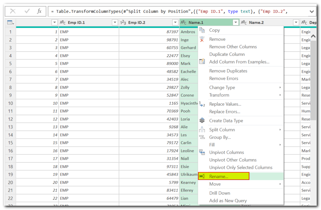
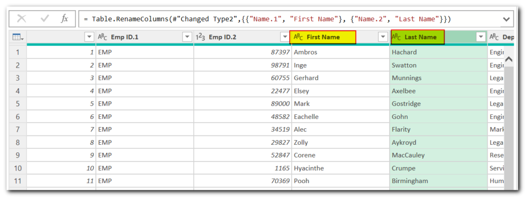
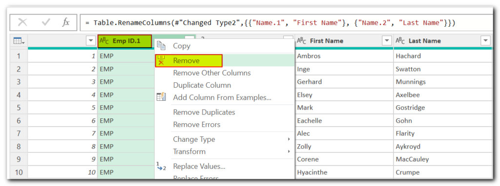
After splitting the columns, it’s essential to refine the data for clarity. Rename the split columns accordingly, such as “First Name” and “Last Name” for the name column, and “Employee ID” for the employee ID column. Remove any unnecessary columns to streamline the dataset.
Step 6: Saving and Loading the Query
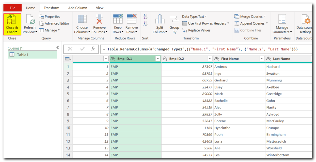
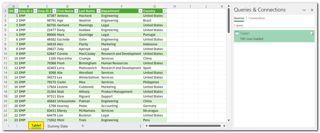
Once the data transformation is complete, click on “Close & Load” to save the query and load the modified data back into Excel. Your refined data will appear in a new sheet, while the original data remains intact as a data source.
Conclusion
By following these step-by-step instructions, you can effectively split data using Power Query in Excel. This powerful feature empowers users to manipulate and organize their data with ease, facilitating better analysis and decision-making processes.
Thank you for exploring this tutorial!


