Sometimes you create amazing projects, dashboards however people can make mistakes and edit the calculations, formats what you have made. Still you can protect the sheets, workbooks and prevent users to make any editing via “Protect Workbook” Option
So here let’s understand how we can do this:

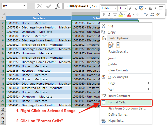
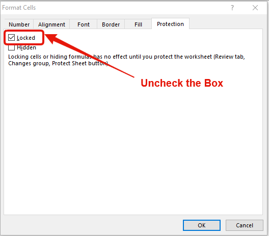
This will unlock the selected Ranges for editing and user may get restricted to these ranges. It will help you to protect your excel formatting, formulas, headers etc. and everybody can use only specified ranges which you may colour code.
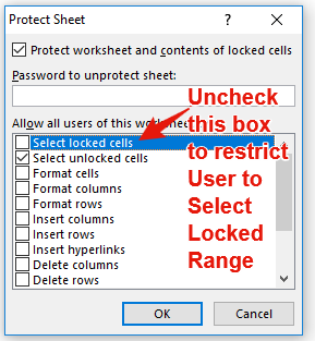
Note: While protecting worksheet, if you uncheck the box “Locked Cells” as below image. It will restrict the user to navigate only on “Unlocked Ranges”
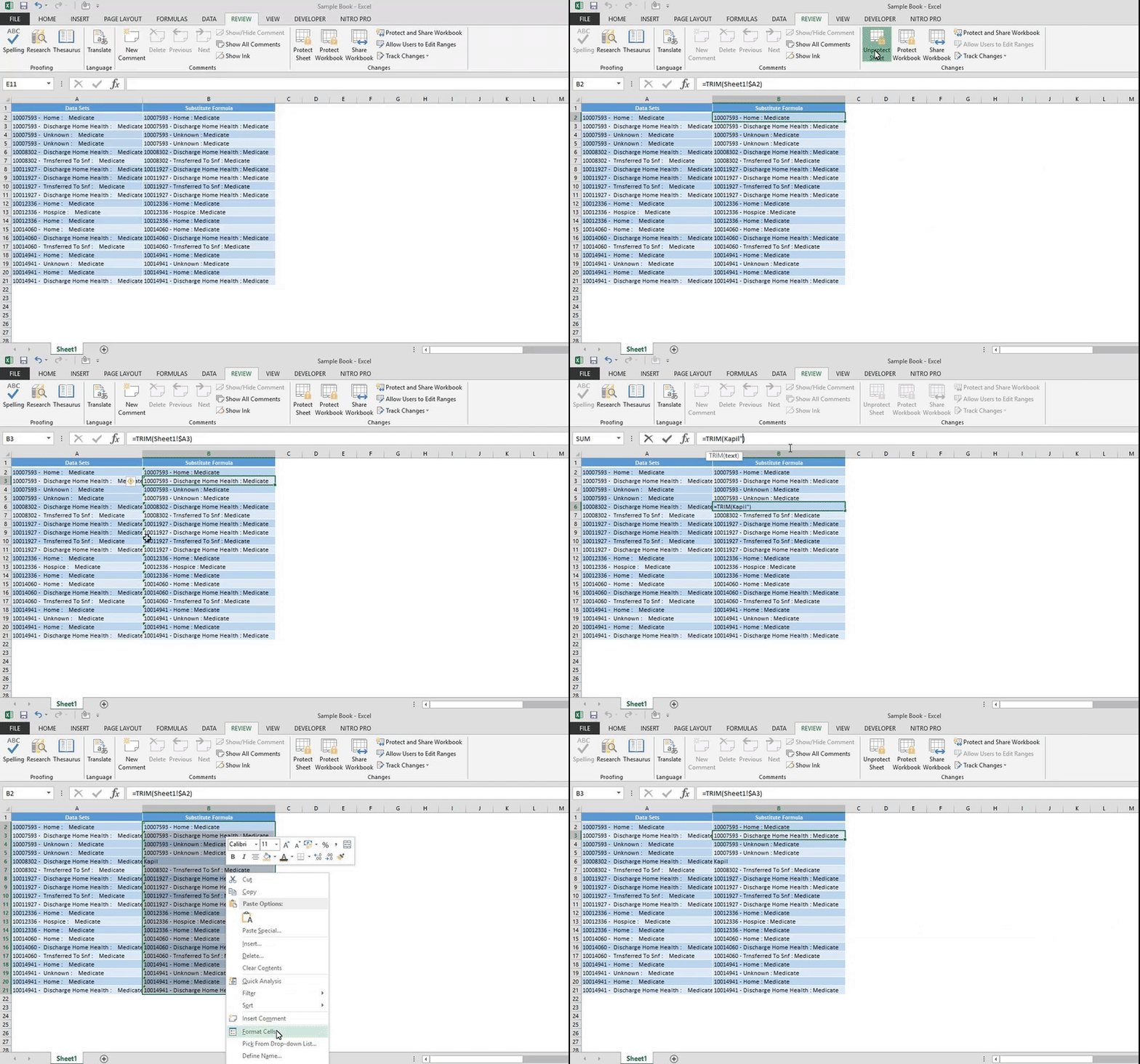
So below gif Image may help you to understand entire process of “Unlocking Specific Range”

Though you can hide Formula Bar but still you can hide formulas without hiding the Formula Bar:
So very simple step, you should follow
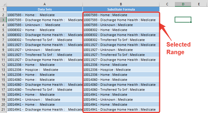

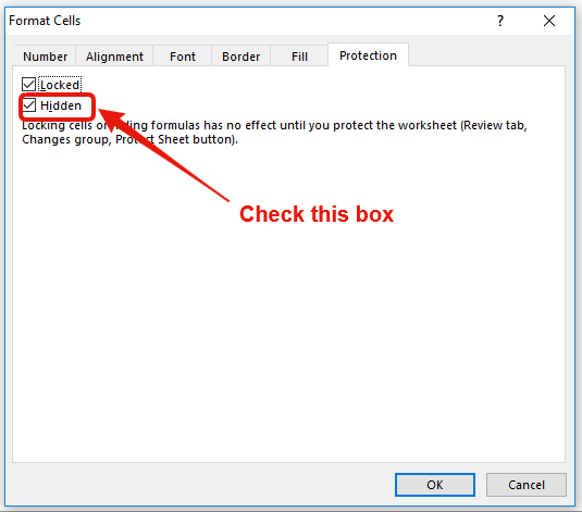
Now when you protect the worksheet, it will hide all the formulas where you have ticked this box.
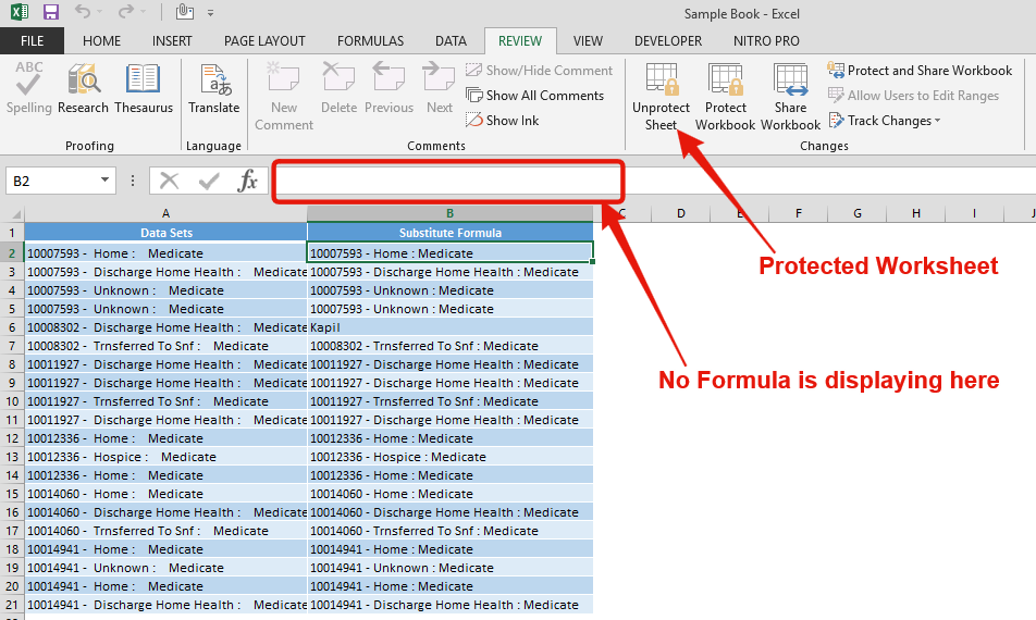
So below gif Image may help you to understand entire process of “Hide Formulas”
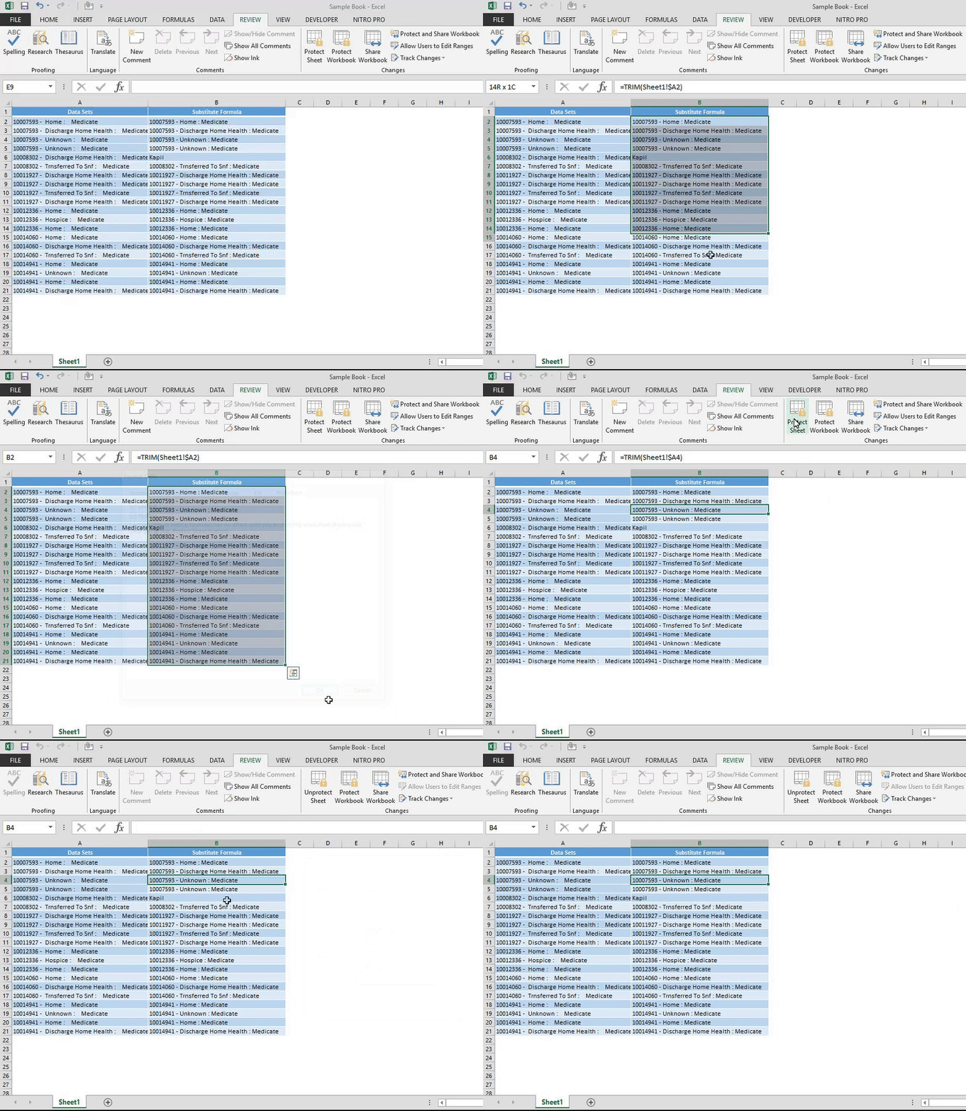
Hope you like but still you have questions or any feedback. Please comment below and share with your friends
When creating a formula in Excel, many people get confused by the $ symbol in cell references. But it’s actually very simple. The dollar sign in an Excel cell reference tells Excel whether to keep the reference the same or allow it to change when you copy the formula to other cells. This guide will explain how it works and why it’s helpful.
Understanding Excel cell references is really important. Knowing the difference between absolute, relative, and mixed references will help you get the most out of Excel formulas and functions.
This tutorial shows you how to change the row colors in Excel to automatically highlight every other row or every nth row or column in your worksheets. You will also learn how to use Excel’s banded rows and columns and find some helpful formulas to shade rows based on value changes.
Using alternating colors for rows in Excel is a common way to make data easier to read. While it’s simple to manually highlight rows in a small table, it can be very time-consuming in larger tables. A better approach is to automatically alternate the colors of rows or columns, and this article will show you how to do it quickly
You need to know how to insert and use the degree symbol in a cell.
Let me explain why this is important. Yesterday, I was working with temperature data, and it was crucial to use the degree symbol to indicate Celsius and Fahrenheit.
Watch: How to use WORKDAY & WORKDAY.INTL Function in Excel? What is WORKDAY Function? The WORKDAY function in Excel calculates a date that is a specified number of working days before or after a given date. It…
This tutorial teaches the basics of correlation in Excel. It shows how to find a correlation coefficient, make a correlation matrix, and understand the results.
Correlation is one of the easiest calculations you can do in Excel. Even though it’s easy, it helps a lot in understanding how two or more things are related. Excel has all the tools you need to do a correlation analysis—you just need to know how to use them
Create Dynamic Data Validation List When I started my career in working with excel dashboards, I always used to face most common challenge in “Data Validation” technique where I want a smart data validation to avoid all…