Microsoft Excel “AND, OR, NOT Functions” are the logical functions and helps to validate the statement if said is “TRUE” or “FALSE”. “AND, OR, NOT” are the three unique logical function and each one of them has their own characteristics.
“AND, OR, NOT Functions” has only one argument i.e. (logical) and multiple logical conditions can be placed in one function. It is easy to apply for validation and output is also very to understand i.e. “TRUE” and “FALSE”. We can place multiple logical conditions in one logical statement.
Output result of “AND” function will be “TRUE” if ALL the logical conditions of a logical statement are correct or matching as per parameters otherwise output result will be “FALSE”.
Output result of “OR” function will be “TRUE” if ANY of the logical condition from a complete logical statement is correct or matching as per parameters otherwise output result will be “FALSE”.
Output result of “NOT” function will be “TRUE” if NO logical conditions from a logical statement is correct or matching as per parameters otherwise output result will be “FALSE”.
“AND, OR, NOT Functions” can be used in various databases whether it is Numeric/Alpha (Strings) etc. which makes the function useful and advantageous. Applying the logical function manually (one by one) to validate if logical condition is “TRUE or FALSE” is very difficult and “AND, OR, NOT Functions” helps to apply the function in large database at once and makes the work easy, saves time and increases efficiency.
“AND, OR, NOT Functions” are very useful and can be used in many situations. Like it can be used as follows:
– Preparing Marks summary and providing Grades as per the marks obtained
– Selection of choices from the available multiple options
– Or any other database where there is requirement placing logical conditions then “AND, OR, NOT Functions” can be used
Things to Remember:
“NOT” function can have only one logical condition, whereas “AND, OR” may have multiple logical conditions in one logical statement.
Also, we need to understand the function output. i.e. “TRUE” means logical statement is matching however “FALSE” means logical conditions are not matching. Also ensure that correct cell reference is given otherwise function output and decisions may go wrong.
“AND” Syntax:
=AND(logical1, [logical2], …)
Syntax Description:
logical, argument is used to give the logical condition. We can place multiple logical conditions to check if conditions are TRUE or FALSE.
Example 1: Explore “AND” Function
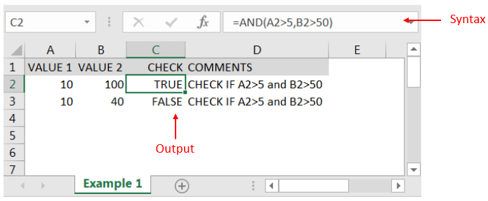
“AND” function’s output will be “TRUE” only incase ALL the conditions are met. As per below example, logical statement is checking for rows# which is greater than 5 and greater than 50. Row#2 meets complete criteria that is why result is “TRUE” whereas Row#3 did not meet the second criteria (i.e. 40 is not greater than 50) that is why output result is “FALSE”
“OR” Syntax:
=OR(logical1, [logical2], ...)
Example 2: Explore “OR” Function
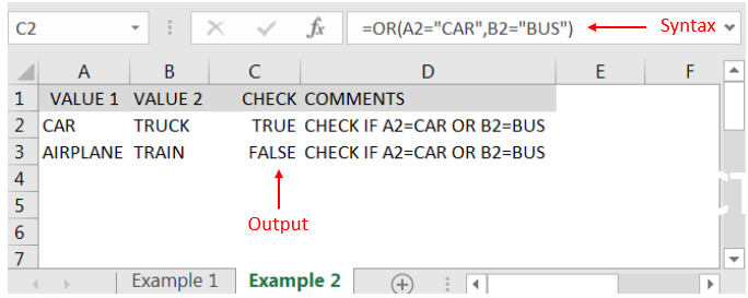
“OR” function’s output will be “TRUE” in case ANY of the following condition is met. As per below example, logical statement is checking for rows# which has either CAR or BUS. Row#2 meets the one criterion out of two that is why result is “TRUE” whereas Row#3 did not meet any of the criteria (i.e. value did not have either CAR or BUS) that is why output result is “FALSE”
“NOT” Syntax:
=NOT(logical1)
Example 3: Explore “NOT” Function
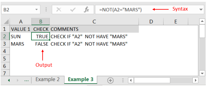
“NOT” function’s output will be “TRUE” in case NO logical conditions in a logical statement is met. As per below example, logical statement is checking for cells# which does not have “MARS”. Cell “A2” meets the criteria (i.e. Cell “A2” is SUN and not MARS”) that is why result is “TRUE” whereas output result of “A3” is “FALSE” (i.e. cell “A3” has “MARS”)
Hope you liked. Happy Learning.
Don’t forget to leave your valuable comments!

Watch Video: Rand and Randbetween Excel Functions Generate Random Numbers using Excel Functions We have got many instances where we needed to generate a random database or values. “RAND function” is very useful for users…

How to use the compound interest formula in Excel and gives examples of how to calculate the future value of an investment with yearly, monthly, or daily interest. It also shows you step-by-step how to make your own Excel compound interest calculator.

UPPER function is used for changing the text/string to UPPER case in Microsoft Excel. The output of the function returns value in new cell.
COLUMNS function is used to get the total count of columns in an array or in cells range for excel worksheet.
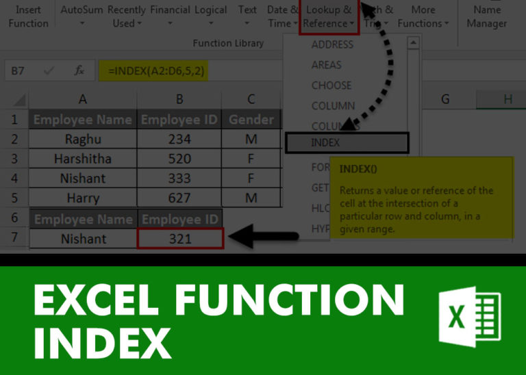
INDEX function is used to get the value from a cell range or table, function returns the value from a table where row and column intersect with each other.

In this tutorial, you will learn 3 effective approaches How to Extract First Line in Excel of text. formulas, regex. In data analysis, Excel is a powerful tool that helps make difficult tasks easier. One…