The AVERAGEIF function is used to get the “average” of values for a range of cells, based on multiple criteria.
The mathematical Average is calculated following: = Sum of all values / (divided by) number of items.
AVERAGEIF Function has two required arguments i.e. range, criteria and optional argument i.e. [average_range].
=AVERAGEIF(range,criteria,[average_range])
range argument is used to give the range of cells in which criteria needs to find
criteria argument is used to give criteria for average. We can give value (example “A”,”A*” >10, 50 ) or cell reference# (example: E2) in this argument
average_range argument is used to give cell range; those values to be averaged as per the criteria mentioned above
Kindly note, [average_range] is optional ONLY incase where range and [average_range] are in ONE column, but if, range and [average_range] are in DIFFERENT columns then [average_range] is NOT optional.
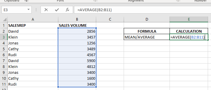
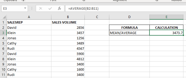
When we want to calculate the average with any condition than AVERAGEIF is used.
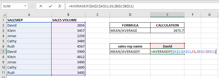
Here in example 2, we are calculating the average sales volume but with 1 condition, that’s why we will use AVERAGEIF here.
Formula:- =AVERAGEIF($A$2:$A$11,E6,$B$2:$B$11)
So here Criteria 1 is sales volume, the condition is David, and criteria 2 is a sales rep.
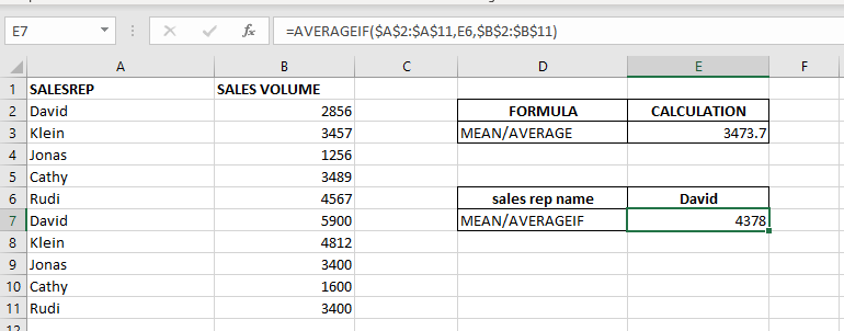
basically, we want to count the average of sales done by David.
The result is 4378 as shown in the 2nd image.
– Criteria argument can also work with Wild characters i.e. asterisk (*), question mark (?). Asterisk will find any series of characters and Question mark will find a single character.
– If you want to search actual * or ? (Asterisk or Question Mark) then type tilde (~) before * or ?
Hope you learnt this Function,
Don’t forget to leave your valuable comments!
If you liked this article and want to learn more similar tricks, please Subscribe us or follow us on Social Media by clicking below buttons:
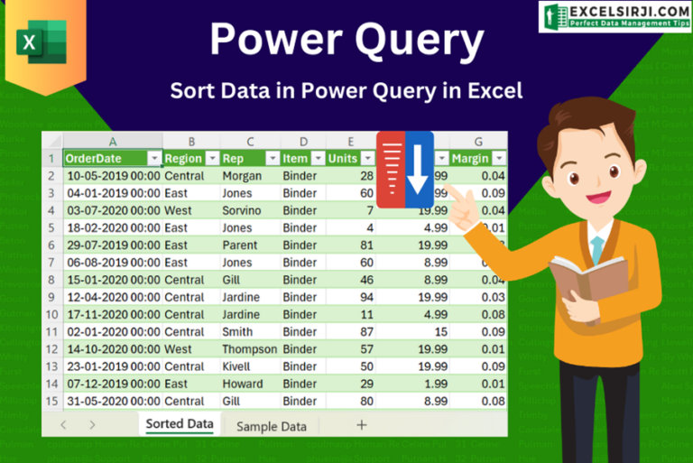
This article unveils the magic of Power Query, a built-in Excel tool that simplifies data organization. Learn how to sort by single or multiple columns, create layered sorts for complex needs, and even reverse your data order entirely. Power Query puts you in control, transforming your data into a well-structured format for effortless analysis.
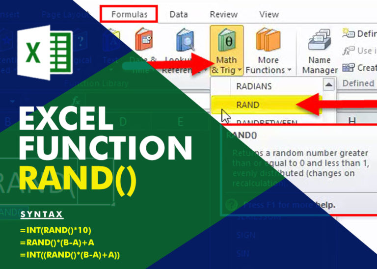
Generate Random Numbers in Excel Using RAND We have got many instances where we needed to generate a random database or values. Rand function is very useful for the users who creates random database for…
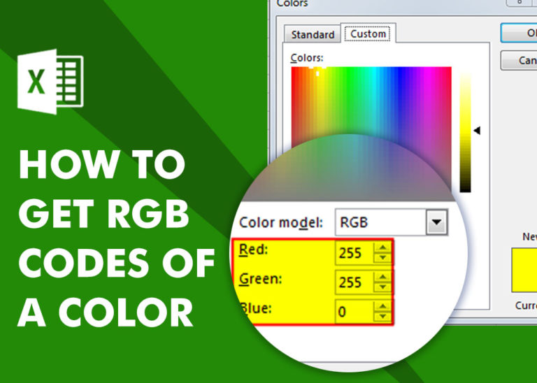
How to Get RGB Codes of a Color? Excel supports more than 16 million colors in a cell; hence you should know how to set the exact color in a cell. To do this through…

Microsoft Excel is a useful tool for analyzing data and conducting statistical research. The program includes numerous functions for performing various statistical calculations. One of the essential measures Excel supports is the weighted average.

The ROMAN function in Excel converts numbers into Roman numerals. It’s useful when you need to display numbers in the Roman numeral format, such as for dates, titles, or other specific purposes. The function allows you to choose how “traditional” or simplified the Roman numeral should be. To use the ROMAN function, you just need to enter the number you want to convert, and Excel will do the rest

In this tutorial, we will explore the CHOOSEROWS function in Excel 365 and how to use it in real life. Imagine you have a big Excel sheet with hundreds of rows, and you need to…