Watch Excel Tutorial Video – Excel Function – AVERAGEIFS
How to use “AVERAGEIFS” function in Excel
AVERAGEIFS function is used to get the “average” of values for matching criteria across range.
Mathematical Average is calculated following : = Sum of all values / (divided by) number of items
AVERAGEIFS Function has required arguments i.e. average_range, criteria_range1, criteria1 and Optional arguments i.e. [criteria_range2, criteria2]… We can place add more than one range to include multiple criteria or conditions.
Syntax:
=AVERAGEIFS(average_range,criteria_range1,criteria1,[criteria_range2,criteria2]…)
Syntax Description:
average_range argument is used to give range/ list of values to calculate average as per below criteria
criteria_range1 argument is used to give the range in which criteria1 needs to find
criteria1 argument is used to give criteria for average. We can give value (example “A”, >10, 50) or cell reference number in this argument
[criteria_range2] optional argument is used to give the ANOTHER range in which criteria2 needs to find
[criteria2] optional argument is used to give criteria2 for average. Value or cell reference number can be given.
Kindly note, we can add multiple criteria in the function by separating them with Comma ( , )
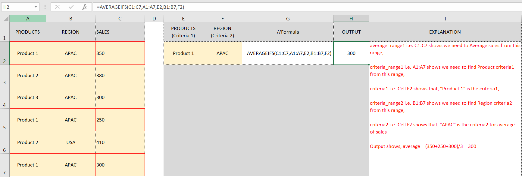
Example 1: AVERAGEIFS function with Multiple Criteria:
- “Column A to C” has Sales details,
- “Column E” shows the sample criteria1,
- “Column F” shows the sample criteria2,
- “Column G” shows the sample formula applied,
- “Column H” shows the output of the function and,
- Explanation is provided in Column “I”

Don’t forget to leave your valuable comments!
If you liked this article and want to learn more similar tricks, please Subscribe us.


