We have got many instances where we needed to generate a random database or values. Rand function is very useful for the users who creates random database for various types of working and analysis.
Rand Function generates values between 0 to less than 1. We always have output of the Rand function in decimals. The formula of RAND function is very simple because it has no arguments and provides the random output.
Below are the RAND Formula syntax commonly used in Excel:
1. =RAND() RAND Function can be used to get the values in decimals, without decimals, values in pre-defined range, we will all discuss in following examples:
Suppose we need to create a database for the various types of stationery products and their prices for a month. There is one way to mention the random product name and prices one by one or we can use the “RAND” function to make the work easy. Here we will go ahead with using RAND Function:
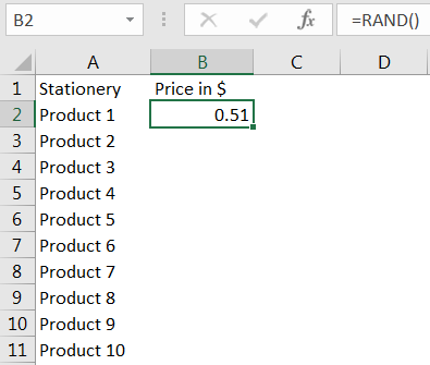
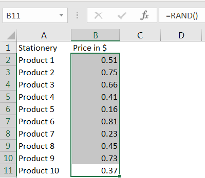
Drag the formula to respective cells. i.e. Select Column + Ctrl + D
If we need to have the random values without decimal, we need to follow the below function. We can have any range based on the requirement; here we need the random values between 0 to 10.
Syntax: =INT(RAND()*10)
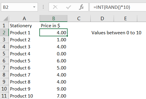
Above syntax will help to get the random values between 0 to 10. If we need to have values between 0 to 100, we will change the syntax and will mention 100 instead of 10
Syntax has limitation that it always gives values starting from 0, if we need to have values within user defined range follow the Example 3.
Suppose we need the random values between a range, between 10 to 100 then please follow below equation, where “b” can be 100 and “a” would be 10
Syntax =RAND()*(b-a)+a
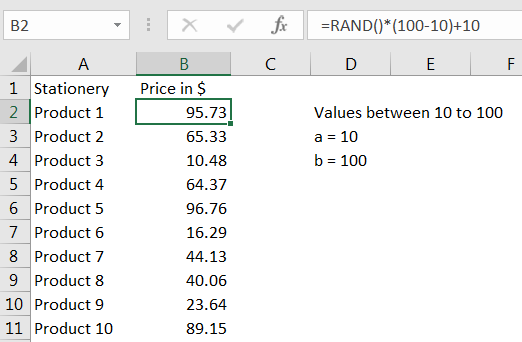
Above function output always returns the value as per the value of “a” and “b” given in the formula. We can give any value in place of 10 or 100 to get the desired result.
We can also have the values between a user defined range and without decimals by following below syntax. For example, if we need the values between 10 to 100:
Syntax: =INT((RAND()*(b-a)+a))
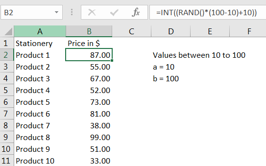
Things to Remember:
– Values derived from RAND function changes each time worksheet is refreshed/ edited/open/changed. So, ensure to Paste special values the formula output so that database is not changed.
Below are the steps for paste special database to values:
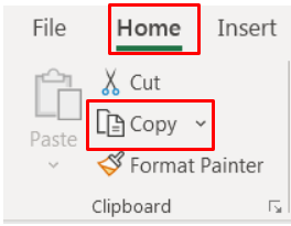
– Select the data range -> Go to Menu Bar- > Click to Home-> Click to Copy
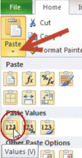
Then -> Go to Menu Bar- > Click to Home-> Click Paste Values
Hope you learnt this Function! you may comment in below comment box for any questions regarding this formula.
If you are liking our articles and want to learn more similar tricks, please do not forget to Subscribe us or follow us on Social Media.
INDEX function is used to get the value from a cell range or table, function returns the value from a table where row and column intersect with each other.

Excel Function COUNTIF COUNTIF Excel Function is also one of the most used function in excel. This helps the user to calculate the number of counts based on single logic given by the user. You…

How to count words in Excel using the LEN function along with other Excel functions. It also gives formulas for counting words or text, whether case-sensitive or not, in a cell or range.

In an “IF function” there will be two output i.e. TRUE or FALSE since either the statement will be “TRUE” or “FALSE”. If the statement is matching or correct, then output will be “TRUE” or if the statement is not matching or not correct then the output will be “FALSE

“NETWORKDAYS” function is very helpful feature in the Microsoft excel to calculate the working days from a particular period excluding “Saturday and Sundays”. NETWORKDAYS function subtract the Start Day from the End Date provided.

COUNT function is used to get the total count of Number values in range or list.COUNT Function has one required and optional arguments.