The AVERAGEIF function is used to get the “average” of values for a range of cells, based on multiple criteria.
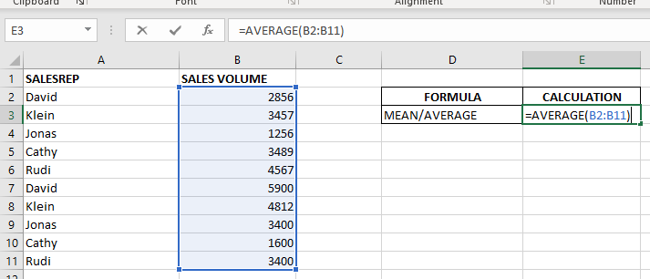
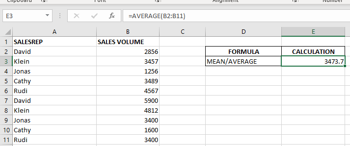
The mathematical Average is calculated following: = Sum of all values / (divided by) number of items.
AVERAGEIF Function has two required arguments i.e. range, criteria and optional argument i.e. [average_range].
=AVERAGEIF(range,criteria,[average_range])
range argument is used to give the range of cells in which criteria needs to find
criteria argument is used to give criteria for average. We can give value (example “A”,”A*” >10, 50 ) or cell reference# (example: E2) in this argument
average_range argument is used to give cell range; those values to be averaged as per the criteria mentioned above
Kindly note, [average_range] is optional ONLY incase where range and [average_range] are in ONE column, but if, range and [average_range] are in DIFFERENT columns then [average_range] is NOT optional.
When we want to calculate the average with any condition than AVERAGEIF is used.
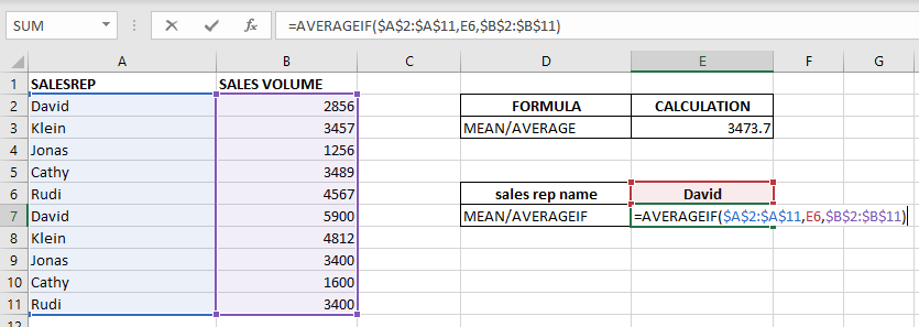
Here in example 2, we are calculating the average sales volume but with 1 condition, that’s why we will use AVERAGEIF here.
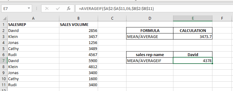
Formula:- =AVERAGEIF($A$2:$A$11,E6,$B$2:$B$11)
So here Criteria 1 is sales volume, the condition is David, and criteria 2 is a sales rep.
basically, we want to count the average of sales done by David.
The result is 4378 as shown in the 2nd image.
– Criteria argument can also work with Wild characters i.e. asterisk (*), question mark (?). Asterisk will find any series of characters and Question mark will find a single character.
– If you want to search actual * or ? (Asterisk or Question Mark) then type tilde (~) before * or ?
Hope you learnt this Function,
Don’t forget to leave your valuable comments!
If you liked this article and want to learn more similar tricks, please Subscribe us or follow us on Social Media by clicking below buttons:

Excel Function REPLACE REPLACE function is used to replace the existing text from a specific location in a cell to New Text. REPLACE Function has argument four arguments i.e. old_text, start_num, num_chars and new_text. We need to give the…

LEFT function is used for extracting the “Left Most” characters from the available string. The output of the function returns the extracted characters in new cell
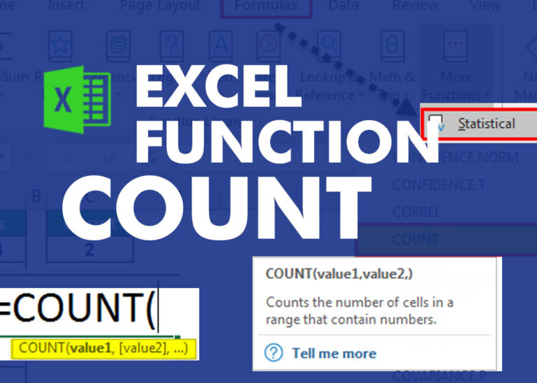
COUNT function is used to get the total count of Number values in range or list.COUNT Function has one required and optional arguments.

Microsoft Excel “NOW” function is used to get the current Date and Time. It is very useful function and can be used in many ways.

LEN function is used for counting number of characters in available string. The output of the function returns the count in new cell.

AND, OR, NOT Functions” provide result in “TRUE” or “FALSE”. If the logical condition is correct and matching the parameters provided, then result would be “TRUE” or if logical condition is not correct and not matching the parameters provided then result would be “FALSE”