FIND function is used to locate the position of text, or character in an available string.
FIND Function has argument two required arguments i.e. find_text, within_text and one optional argument i.e. [start_num]. If no value is provided in [start_num] argument then function will take the Default value i.e. 1
=FIND(find_text, within_text, [start_num])
find_text argument, is used to give text, character or cell reference that is required to find
within_text argument, is used to give the cell reference from which text (i.e. find_text value ) to be searched
[start_num] is optional argument and is used to specify the character from which search should start. By default, the first character is 1, however if you want search should be started from 2nd find_text value then it should be position of 2nd find_text value and so on..
Here we have some examples, where:
– “Column A” has various strings,
– “Column B” shows the sample formula that is applied,
– “Column C” shows the output of the function and
– Explanation is provided in “Column D

– Output in Cell “C2” i.e. “6” is showing that the character “u” is available at “once upon” and “u” has 6th position.
– Output in Cell “C3” i.e. “13” is showing that the character “T” is available at “Tree” and has 13th position. Also note that character “t” is ignored in “there”
– Output in Cell “C4” i.e. “8” is showing that the character “t” is available at “tree” after ignoring character “t” at “that”.
– Find function is case sensitive, means it will only search “t” for text “the” and not with “The”. If you want to find value without case sensitive, then try “SEARCH” Function
– Find function will not work with Wild characters i.e. asterisk (*), question mark (?)
– Function should give output in “General” format, however if output is not as per the desired format then we need to change the cell format to “GENERAL”.
– If function parameters are not correctly applied in the function, then it will give output as “#VALUE!” (Error).
Don’t forget to leave your valuable comments!
If you liked this article and want to learn more similar tricks, please Subscribe us

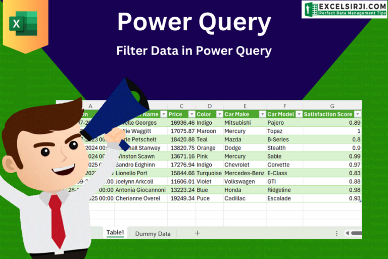
This step-by-step tutorial empowers you to leverage Power Query’s robust filtering capabilities. Learn to filter by date, text, numbers, and more, streamlining your workflow and unlocking deeper insights from your data. Watch now and elevate your Excel expertise!

AVERAGEIF function is used to get the “average” of values for matching criteria across range. Average = Sum of all values / number of items.

Unhide Cells in Excel means you’ve probably hidden a row, column, or worksheet before to focus on important data. But what if you need to see those hidden parts again? Don’t worry—Excel makes it easy…

How to use the compound interest formula in Excel and gives examples of how to calculate the future value of an investment with yearly, monthly, or daily interest. It also shows you step-by-step how to make your own Excel compound interest calculator.

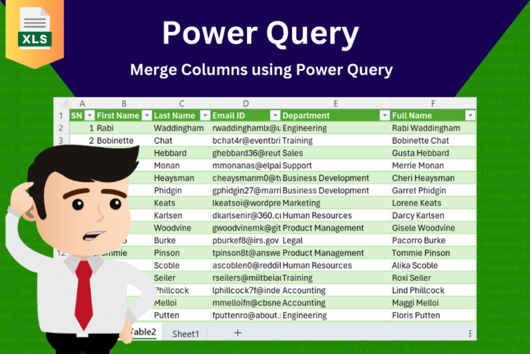
In this tutorial, learn how to merge columns using Power Query. Follow this step-by-step guide to convert data into a table, merge columns seamlessly, and customize separators. Whether you’re a beginner or an advanced user, this tutorial will enhance your data manipulation skills and streamline your workflow. Master Power Query and optimize your data management processes effortlessly.

What is Strikethrough in Excel? Strikethrough in Excel is a feature that lets you draw a line through text. It’s like crossing something out, usually to show that it’s no longer needed or has been…