FIND function is used to locate the position of text, or character in an available string.
FIND Function has argument two required arguments i.e. find_text, within_text and one optional argument i.e. [start_num]. If no value is provided in [start_num] argument then function will take the Default value i.e. 1
=FIND(find_text, within_text, [start_num])
find_text argument, is used to give text, character or cell reference that is required to find
within_text argument, is used to give the cell reference from which text (i.e. find_text value ) to be searched
[start_num] is optional argument and is used to specify the character from which search should start. By default, the first character is 1, however if you want search should be started from 2nd find_text value then it should be position of 2nd find_text value and so on..
Here we have some examples, where:
– “Column A” has various strings,
– “Column B” shows the sample formula that is applied,
– “Column C” shows the output of the function and
– Explanation is provided in “Column D

– Output in Cell “C2” i.e. “6” is showing that the character “u” is available at “once upon” and “u” has 6th position.
– Output in Cell “C3” i.e. “13” is showing that the character “T” is available at “Tree” and has 13th position. Also note that character “t” is ignored in “there”
– Output in Cell “C4” i.e. “8” is showing that the character “t” is available at “tree” after ignoring character “t” at “that”.
– Find function is case sensitive, means it will only search “t” for text “the” and not with “The”. If you want to find value without case sensitive, then try “SEARCH” Function
– Find function will not work with Wild characters i.e. asterisk (*), question mark (?)
– Function should give output in “General” format, however if output is not as per the desired format then we need to change the cell format to “GENERAL”.
– If function parameters are not correctly applied in the function, then it will give output as “#VALUE!” (Error).
Don’t forget to leave your valuable comments!
If you liked this article and want to learn more similar tricks, please Subscribe us

Many tasks in Excel require comparing data in different cells. To do this, Excel offers six logical operators, also known as comparison operators. This tutorial will help you understand how these operators work and how to write efficient formulas for data analysis

MOD function is used to get the remainder of number that is divided by divisor. MOD Function has two required arguments i.e. number and divisor.

How to Create a Pivot Table? Pivot Tables in excel is backbone of data analysis in excel. If you want to perform various analysis in excel, then I would suggest, learn this amazing excel feature…

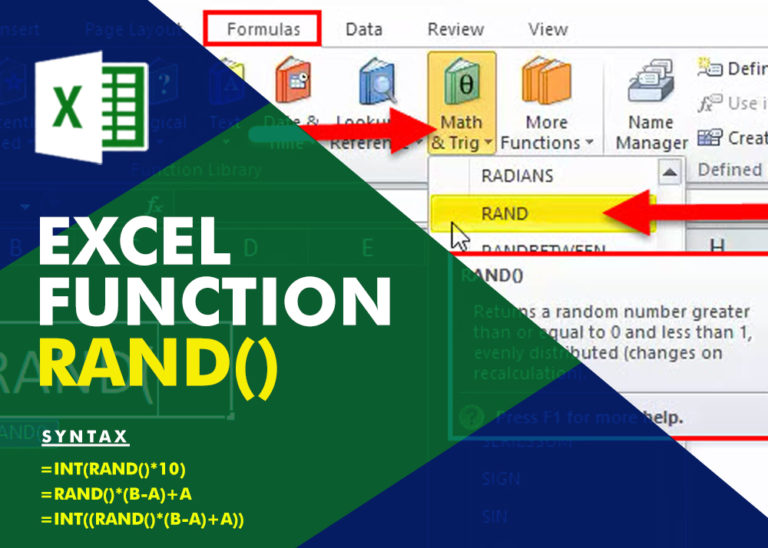
Generate Random Numbers in Excel Using RAND We have got many instances where we needed to generate a random database or values. Rand function is very useful for the users who creates random database for…

This tutorial explains how to use the IFERROR function in Excel to catch and handle errors. It shows you how to replace errors with a blank cell, a different value, or a custom message. You’ll also learn how to use IFERROR with functions like VLOOKUP and INDEX MATCH, and how it compares to other error-checking functions like IF ISERROR and IFNA

In this tutorial, you will learn how to make your daily tasks easier and quickly understand your data using the Excel Quick Analysis tool. Microsoft Excel is a powerful program that helps you work with…