Microsoft Excel “ISERROR Function” is a Logical Function and it is used to check if cell contains any “ERROR”. “ISERROR Function” is used as a test to validate if cell contains any Error or not.
“ISERROR Function” has only one argument i.e. (value) and it is easy to apply for validation of cell, it provides the output that is easy to understand i.e. “TRUE” and “FALSE”
“ISERROR Function” can be used in any type of databases or cells whether it is Numeric/Alpha (Strings) etc. which makes the function useful and advantageous. Applying the logical function manually (one by one) to validate if cell has any “ERROR” or “NON-ERROR” is very tedious and “ISERROR Function” helps to apply the function in large database at once and makes the work easy, saves time and increases efficiency.
“ISERROR Function” is very useful and can be used in multiple situations. Like it can be used as follows:
– Large excel worksheet which has many formulas placed
– Or any other database where there is requirement of validation of cells if any of cell contains any “Error” or not then “ISERROR Function” can be used
Syntax:
=ISERROR(value)
Syntax Description:
value, argument is used to give the cell reference. It is the cell number that is to be checked for “ERROR”
Things to Remember:
We need to understand the function output. If cell contains any “ERROR” then output will be “TRUE” or if cells contains “NO ERROR” then output will be “FALSE”
ISERROR function will work with any of the excel errors such as #REF!, #N/A, #VALUE!, #DIV/0!, #NUM!, #NULL!, or #NAME?
Also ensure that correct cell reference is given otherwise function output and decisions may go wrong.
Example 1: Validation of Large excel Database
Suppose we have employee database where address fields need to be validated if any of cell contains any error. We can utilize this function as follows:
Syntax: = ISERROR(B2)

We can review the above results that cells “A2” and “B2” contains excel errors i.e. #REF! and #NA that is why the output in cell “B2” and “C2” are “TRUE”. Whereas cells “A4” to “A7” does not contains any errors that is why the output in cells “B4” to “B7” are “FALSE”
Likewise, we can apply the “ISERROR Function” whenever there is requirement of validation of “Errors”
Hope you liked. Happy Learning.
Don’t forget to leave your valuable comments!

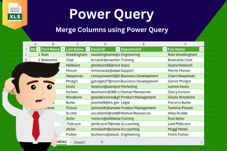
In this tutorial, learn how to merge columns using Power Query. Follow this step-by-step guide to convert data into a table, merge columns seamlessly, and customize separators. Whether you’re a beginner or an advanced user, this tutorial will enhance your data manipulation skills and streamline your workflow. Master Power Query and optimize your data management processes effortlessly.

In this tutorial, we’re going to explore one of the most intriguing features in Excel: the OFFSET function.
So, what is the OFFSET function in Excel? Simply put, OFFSET gives you a reference to a range of cells that’s moved from a starting point by a certain number of rows and columns.

Watch Excel Tutorial Video – How To Create Dropdown List In Excel How to Create a Dropdown list in excel? Microsoft Excel is what most professionals are using for their day-to-day office. Creating a drop-down…

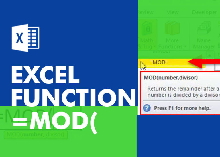
MOD function is used to get the remainder of number that is divided by divisor. MOD Function has two required arguments i.e. number and divisor.

Watch: How to use VLOOKUP Function in Excel? What is VLOOKUP Function? The VLOOKUP function in Excel searches for a value in a table and returns a corresponding value from another column in the same row…

Microsoft Excel “ISBLANK Function” is a Logical Function and it is used to check if cell in question is “BLANK OR NON-BLANK”. “ISBLANK Function” is used as a test to validate if cell contains any…