The objective of creating drop-down list is to give an option to a user to select the option from the list.
so that it restricts the user to select unwanted entries input.
we can also use drop-down option for creating interactive dashboards for reporting purpose.
STEP 1 :- As we can see on the top we have a data entry form at the bottom we have a dashboard
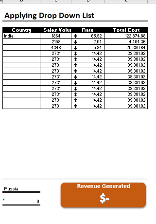
STEP 2 :- So for creating a drop-down list select a cell and go to data under this data there is data validation icon.
now click on the data validation and the screen will pop up shown below.
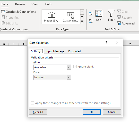
STEP 3 :- Now under the setting option click the allow button and select the list. now in source write the entries for eg india, united states, china etc we can add as many countries than click ok.
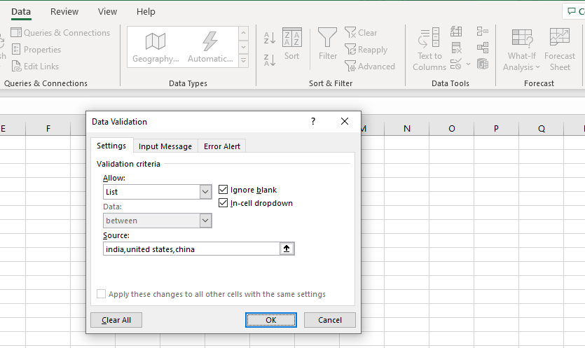
STEP 4 :- Now after this, if we select any cell there is a dropdown list of entries like India,united states, china, etc. so our drop-down list is updated.
Now let us understand how to create a drop-down from the list because whenever we have big data sets than it is not easy to write manually every entry. In this case, We will follow the steps given below.
Step 1: Select the cells containing the headings and values
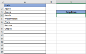
Step 2: Click on “Data” on the top of excel and select Data Validation:

Step 3: Select List under “Allow” and enter the Range of your data under “Source”. Click Ok:
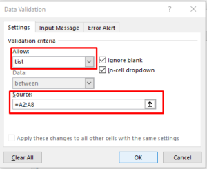
Note: In order to fix the range, you need to use “$” sign before Column and Row reference values i.e. $A$2:$A$8
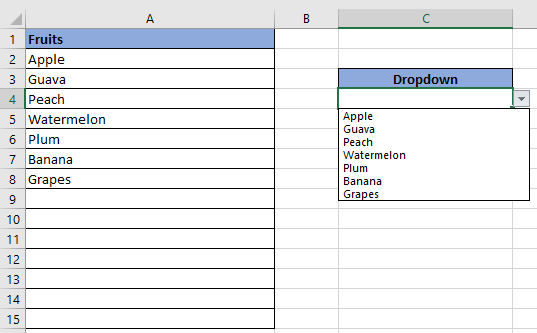
Step 4: Here is your drop down list:

Microsoft Excel “NOW” function is used to get the current Date and Time. It is very useful function and can be used in many ways.

The ROMAN function in Excel converts numbers into Roman numerals. It’s useful when you need to display numbers in the Roman numeral format, such as for dates, titles, or other specific purposes. The function allows you to choose how “traditional” or simplified the Roman numeral should be. To use the ROMAN function, you just need to enter the number you want to convert, and Excel will do the rest

This tutorial explains how the TRANSPOSE function works and shows you the right way to use it to switch data in Excel.
Everyone has different preferences, even for work habits. Some people like to arrange data in vertical columns, while others prefer horizontal rows. If you ever need to switch the direction of your data quickly, the TRANSPOSE function can help
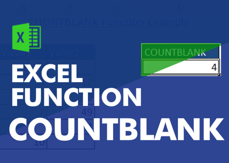
COUNTBLANK function is used to get the total count of Blank or Empty cell in range.
COUNTBLANK Function has one required argument i.e. range.
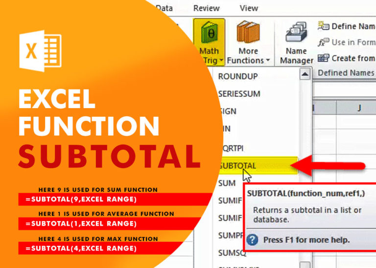
Excel Function SUBTOTAL Excel Function “Subtotal” is most commonly used formula in excel and it can make your work easy while performing simple mathematical calculations because of variety of features like: – You can use…
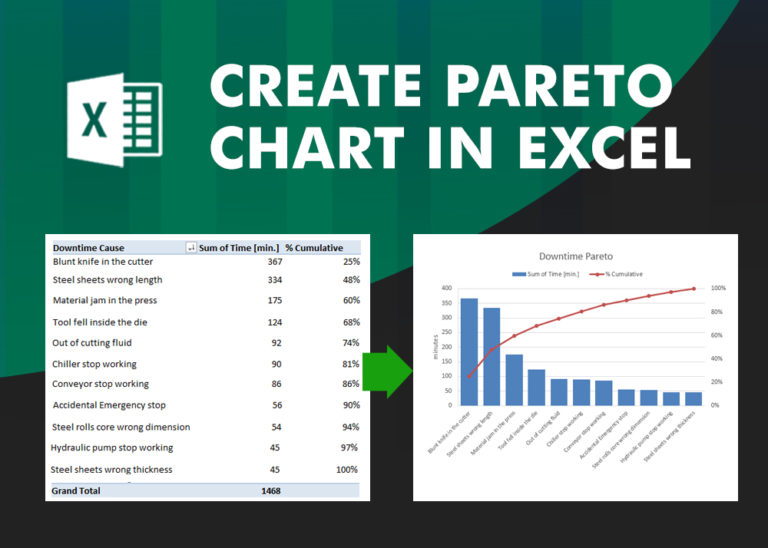
What is Pareto Chart? Pareto principle was introduced by Italian Economist Vilfredo Pareto. He stated that 80% of the effects are caused by 20% of the causes. So if we closely monitor and solve 20% of…