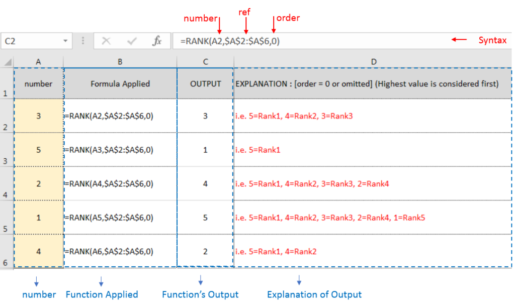
RANK function performs the Ranking in a range or list of numbers. Function returns the rank position and can assigned as Highest or Lowest value as 1st rank as per order argument.
Syntax:
=RANK(number,ref,[order])
number argument is used to give number value for which ranking is required
ref argument is used to give range or list of values from which rank to measure
[order] is optional argument and Value 0 or 1 can be given as per below requirements:
[order] = 0 or omitted: Highest value will be Ranked as 1st position (example: Value 5=Rank1, 4=Rank2, 3=Rank3, 2=Rank4, 1=Rank5 and so on)
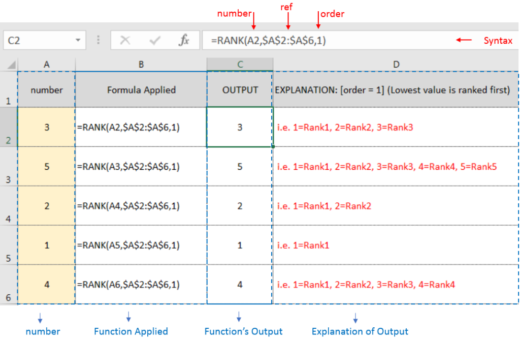
[order] = 1: Lowest value will be Ranked as 1st position (example: Value 1=Rank1, 2=Rank2, 3=Rank3, 4=Rank4, 5=Rank5 and so on)

Example 2: RANK function with [order = 1] (Lowest value is ranked first)

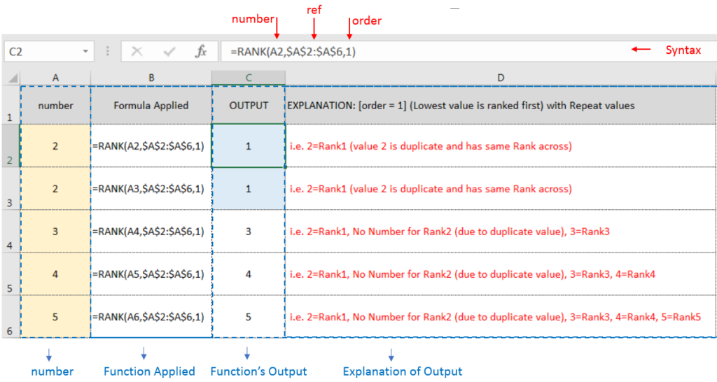
Example 3: RANK function with [order = 1] (Lowest value is ranked first) with Repeat values

If list of values or ref argument has duplicate values, ranking for those values will be same across
Hope you learnt this Function,
Don’t forget to leave your valuable comments!
If you liked this article and want to learn more similar tricks, please Subscribe us or follow us on Social Media by clicking below buttons:

SEARCH function is used to find “position of character or text” in an available cell and this function is NOT case sensitive.

In this tutorial, learn how to merge columns using Power Query. Follow this step-by-step guide to convert data into a table, merge columns seamlessly, and customize separators. Whether you’re a beginner or an advanced user, this tutorial will enhance your data manipulation skills and streamline your workflow. Master Power Query and optimize your data management processes effortlessly.

WORKDAY Function in Excel Are you working today? or Do you have Work Off or holiday today? I am asking this question because I am gonna tell you the most commonly used function in Excel…

SUM Function in Excel Excel is a mathematical spreadsheet where you can perform multiple calculations with the help of Excel Formulas. These are automated formulas which refreshes automatically once you refresh your data in a…

To subtract numbers in Excel, follow these steps:
Start by typing an equal sign (=) in the cell where you want the result.
Enter the first number or cell reference you want to subtract from.
Type a minus sign (-).
Enter the second number or cell reference you want to subtract.

If you want to print your Excel spreadsheets with gridlines, this guide is for you. Adding gridlines makes your data easier to read and gives your spreadsheet a clean, organized look. In this post, we’ll…