Excel is a mathematical spreadsheet where you can perform multiple calculations with the help of Excel Formulas. These are automated formulas which refreshes automatically once you refresh your data in a given range. Here you should know about “Excel Ranges” before starting to use Excel Formulas.
You can SUM (Add) multiple numbers in a given range of excel and get the total amount with just few clicks. So Let’s learn this most basic Excel formula
1. =SUM(Range1,Range2……)2. =SUM(Range1,Range2……)3. =SUM(Range Start:Range End) i.e. =SUM(A2:A4) This formulas can be used to calculate the total of any range/cell reference given in excel. We can use multiple range to find the Total/Sum of given values or we may enter/select values to get the total.
So if you do simple math 2+2=4, you may use this formula to do the same in excel
Things To Remember
– This formula should strictly be used with Numbers only
– If this formula is showing #Ref error, it means that you have deleted or added a Row
– If this formula is showing #N/A error, it means that your range might contain text
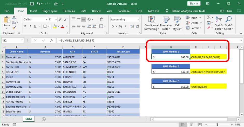
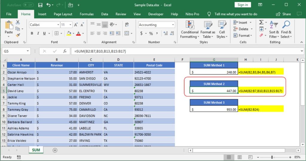
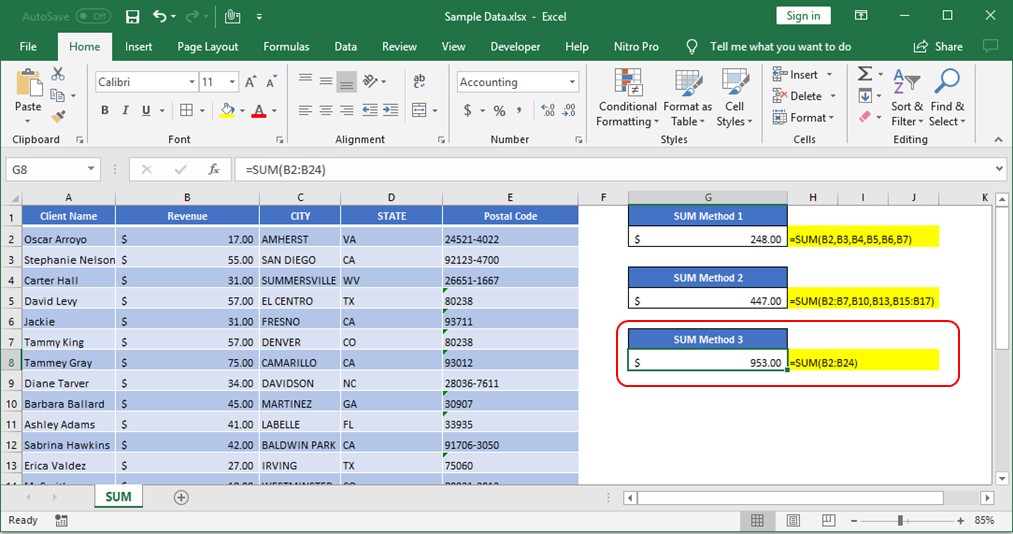
All above mentioned formulas are using the relative references which means that these are dynamic ranges, so if you copy these formulas or paste it somewhere else or drag in rows or columns, ranges will be automatically updated relatively.
So when your Excel Ranges are fixed, you should make excel ranges Fixed/Absolute range. In order to make excel ranges absolute, you can fix those excel range by putting “$” i.e. if you want to fix the columns only, you should use
=Sum($A2:$A10) >> Here we are fixing the column "A" or
=Sum(A$2:A$10) >> Here we are fixing the Rows by putting $ front of 2 and 10
=Sum($A$2:$A$10) >> Here we are fixing both Rows and Columns by putting $

Excel Function- WORKDAY.INTL WORKDAY.INTL function is an advanced version of WORKDAY function with additional advantage of “Custom weekend options” For Example, with WORKDAY function weekends are treated as “Saturday and Sundays” however if you need…
Excel Function REPLACE REPLACE function is used to replace the existing text from a specific location in a cell to New Text. REPLACE Function has argument four arguments i.e. old_text, start_num, num_chars and new_text. We need to give the…

Microsoft Excel “NOW” function is used to get the current Date and Time. It is very useful function and can be used in many ways.

This tutorial teaches the basics of correlation in Excel. It shows how to find a correlation coefficient, make a correlation matrix, and understand the results.
Correlation is one of the easiest calculations you can do in Excel. Even though it’s easy, it helps a lot in understanding how two or more things are related. Excel has all the tools you need to do a correlation analysis—you just need to know how to use them

https://youtu.be/HmJL_y93pAs WEEKNUM function helps to calculate the week number of the given date in a year. It considers 1st January as first week by default and through the output for the given input date. Syntax:…

Microsoft Excel “HOUR, MINUTE, SECOND Functions” are time related functions helps to extract the Hour, Minute or Second from a complete Time.