=TEXT(value,format_text)
value argument [Required] is used to give the text or cell reference for which formatting is to be changed
format_text [Required], is used to give the formatting code as per the requirement
Here we have some examples, where “Column A” has various values, “Column B” represents format_text and “Column C” shows the output of the function.
We will be using TEXT function as follows:
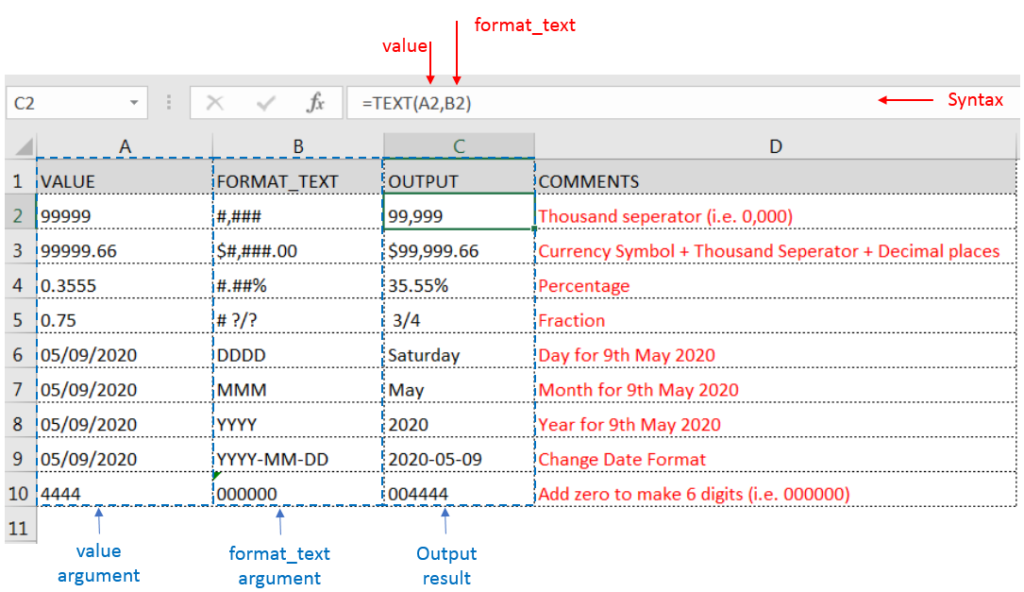
– Format of cell can also be changed by following CTRL+1 (or MAC Command button +1) and select the desired format/appearance
– If cell reference is not correctly provided in the function, then it will give output as an error
– Function should give output in “General” format, however if output is not as per the desired format then we need to change the cell format to “GENERAL”
Hope you learnt this Function,
Don’t forget to leave your valuable comments!
If you liked this article and want to learn more similar tricks, please Subscribe us or follow us on Social Media by clicking below buttons:
Watch: How to use MODE & MODEIF Function in Excel? What is MODE Function? In Excel, the “MODE” function is a statistical tool that identifies and returns the most frequently occurring value within a set…
SUMIFS function is used to get the “total sum” of values for matching criteria across range. SUMIFS Function has required and optional arguments
COUNTBLANK function is used to get the total count of Blank or Empty cell in range.
COUNTBLANK Function has one required argument i.e. range.

RANK function performs the Ranking in a range or list of numbers. Function returns the rank position and can assigned as highest or lowest value as 1st Rank

AVERAGE function is used to get the average of numbers. Function applies formula i.e. average = Sum of all values / (Divided by) number of items.

How to use the compound interest formula in Excel and gives examples of how to calculate the future value of an investment with yearly, monthly, or daily interest. It also shows you step-by-step how to make your own Excel compound interest calculator.