WEEKNUM function helps to calculate the week number of the given date in a year. It considers 1st January as first week by default and through the output for the given input date.
=Weeknum(serial_number,[return_type])
WEEKNUM function helps to calculate the week number of the given date in a year. It considers 1st January as first week by default and through the output for the given input date.
=Weeknum(serial_number,[return_type])
The WEEKNUM uses the following arguments: Serial_number (required argument) – This is an Excel date for which we want to return the week number. When entering the argument, we should enter the date using the DATE function or as a result of other formulas or functions.
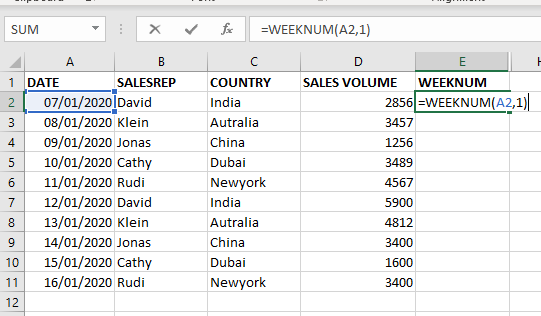
To find the WEEKNUM of the year we use the formula =WEEKNUM(A2,1).
In the WEEKNUM formula select the first argument as date comma now select first day of week it depends every company has different first day of week here i am selecting sunday .
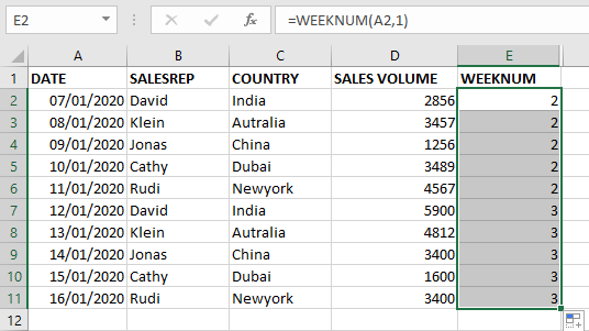
As shown in below image when you apply formula the result is 2 and when we copy formula in column the result is shown in 2nd image.


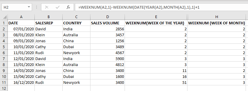
To get week of the month using the same WEEKNUM Formula.
Calculating the week of the year minus the week of the year of first of the same month.
FORMULA=WEEKNUM(A2,1)-WEEKNUM(DATE(YEAR(A2),MONTH(A2),1),1)+1


TEXT function is used to change the formatting or appearances of the text. There are various types of formatting available.

This guide will show you quick and easy methods to find the number of days between dates in Excel.
Do you need to know how many days are between two dates? Maybe you want to find out the days between today and a date in the past or future, or just count the working days between two dates? Whatever you need, one of the examples below will help you find the solution

Discover free videos and tutorials to master Excel formulas and functions. Practice directly in our Online Excel Practice Files without downloading anything. Have questions? Drop them in the comments. Let’s begin! Basic Excel Formulas and…

SUBSTITUTE function is used to substitute the existing old text to new text.

LARGE function is used to get the Largest k-th value from the range.
LARGE Function has two required arguments i.e. array, and k

COLUMN function is used to get the column reference number of the excel worksheet. COLUMN Function has only one argument.