The Microsoft Excel COUNTIFS function counts the number of cells in a range, that meets a single or multiple criteria and adjacent or non-adjacent. As a Statistical function of Excel, the COUNTIFS supports using comparison operators and wildcard characters.

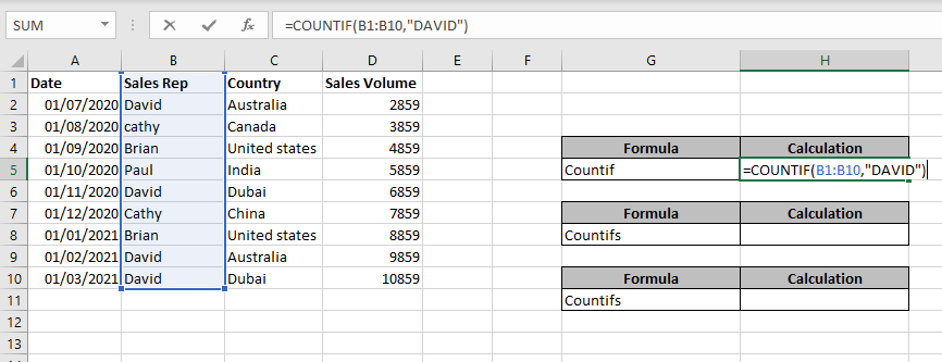
Countif is used to count specific values given in a range of cells.
Formula :-=countif(B1:B10,”DAVID”)
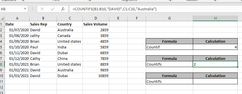
In this example we are counting how many times David are there in sales rep using the formula.
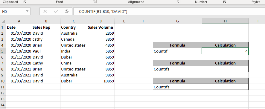
After applying the formula when we press enter it gives us the result. As we can see below pic total count is 4.
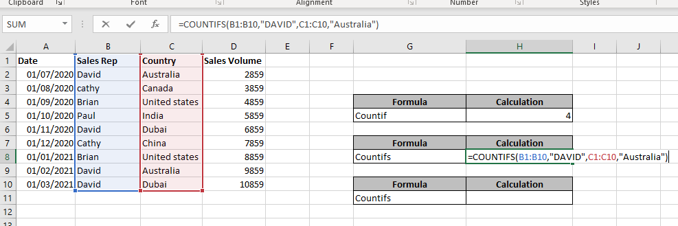
Countifs is used for counting specific value bases on multiple criteria
Formula =COUNTifs(B1:B10,”DAVID”,C1:C10,”Australia”)
In COUNTifs we count a number of cells that contain value with criteria. As we can see in example given below we are counting how many times David did sales in Australia so David’s count is criteria 1 Australia’s count is criteria 2 when we apply the formula and press enter it shows us number 2 as shown below.
Countifs can also be used to count specific values with between, more than, less than criteria as well.
Formula:- =COUNTIFS(B2:B10,”DAVID”,A2:A10,”>=”&”01/07/2020″,A2:A10,”<=”&”01/11/2020″)
In this example, we can see Davids’s sales in a particular country which includes particular dates.. As we can see in the below image we have selected dates and sales reps by applying the formula will get the result of how many times David did sales in Australia from selected dates so the answer is 2 times.


Hope you learnt this Function,
Don’t forget to leave your valuable comments!
This tutorial explains how the TRANSPOSE function works and shows you the right way to use it to switch data in Excel.
Everyone has different preferences, even for work habits. Some people like to arrange data in vertical columns, while others prefer horizontal rows. If you ever need to switch the direction of your data quickly, the TRANSPOSE function can help

The ROMAN function in Excel converts numbers into Roman numerals. It’s useful when you need to display numbers in the Roman numeral format, such as for dates, titles, or other specific purposes. The function allows you to choose how “traditional” or simplified the Roman numeral should be. To use the ROMAN function, you just need to enter the number you want to convert, and Excel will do the rest

SUBSTITUTE function is used to substitute the existing old text to new text.

Microsoft Excel “NOW” function is used to get the current Date and Time. It is very useful function and can be used in many ways.

This tutorial explains what an Excel name is and shows you how to define a name for a cell, range, constant, or formula. You’ll also learn how to edit, filter, and delete defined names in Excel.
Excel names are a bit of a paradox: they’re one of the most useful features, but many people find them unnecessary or too technical. That’s because few users truly understand what Excel names can do. This tutorial will not only teach you how to create a named range in Excel but also show you how this feature can make your formulas easier to write, read, and reuse.

COUNT function is used to get the total count of Number values in range or list.COUNT Function has one required and optional arguments.