EXCEL FUNCTION – MATCH
Video: How to use Excel function MATCH?
Excel Function MATCH
Match function is as same as what it means. Match function helps to match the partial or full user defined value or number in a given range and return the exact or relevant position of the same.
For Example: If we have an array i.e. 1,2,3,4 and if I ask you what is the position of 3 in this array, your answer will be 3rd position in the array. We will explain more examples in details.
Match Function Formula
=MATCH(lookup_value, lookup_array, [match_type])
The MATCH formula uses the following arguments:
- Lookup_value (mandatory argument) – Value which you are going to find in the lookup array. lookup array is your database.
- Lookup_array (mandatory argument) – The database.
Match_type (optional argument) – Match function will helps you to find the location of the lookup value it could be horizontal or it can be vertical. But when you mention horizontal than its horizontal if you mention vertical than its vertical.
Match Excel Function
Let’s look at few examples here to learn more about Excel Function Match
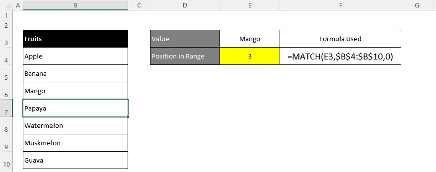
Example 1–EXACT MATCH
Now here we have range “B4:B10” where all fruits are listed. Now on the right side, we have value in E3 cell “Mango” and we want to get the position of Mango in Fruits data given.
Example 2–INDEX MATCH
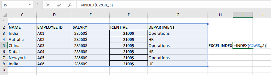
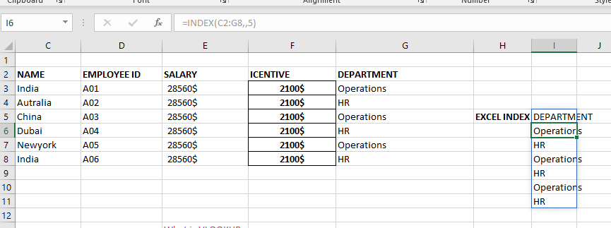
Excel INDEX function is used when you want to pull out the ARRAY RANGE WITH HELP OF formula you can either pull the cell value or you can pull all the AARAY range values with the help of INDEX function.
The formula =INDEX(C2:G8,,5).
In this formula first argument we are selecting