The COUNTA is a cell counting function, which counts all cells in a range that has values, both numbers and letters.
=COUNTA(value1,[value2],...)
value1 argument is used to give any value/ range for which count is required
[value2] argument is used to give another value /cell reference/range
… means, we can add multiple value/cell reference/range by separating them with comma ( , )
The COUNTA function is used when we need to count Non-Blank cells in a selected range.
For example, for counting cells from A1-A10, the formula is “=COUNTA (A1:A10).”
The function also counts the number of value arguments provided. The value argument is a parameter that is neither a cell nor a range of cells.
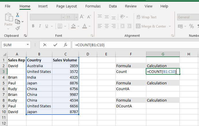
Formula =COUNT(B1:C10) The COUNT Function will count the number of cells with numeric values within the selected range B1 to C10.
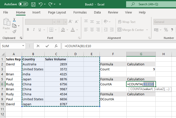
FORMULA =COUNTA(B1:E10
The COUNTA Function will count the number of cells with numeric values and Alpha numeric values within the selected range B1 to E10
Hope you learnt this Function,
Don’t forget to leave your valuable comments!

FIND function is used to find the position of text, or character in an available string.
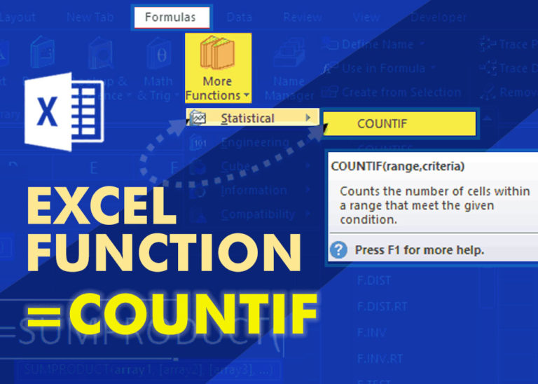
Excel Function COUNTIF COUNTIF Excel Function is also one of the most used function in excel. This helps the user to calculate the number of counts based on single logic given by the user. You…

SUMIF function is used to get the “total sum” for number of times the criteria across range is met. SUMIF Function has two required arguments.

AVERAGEIF function is used to get the “average” of values for matching criteria across range. Average = Sum of all values / number of items.
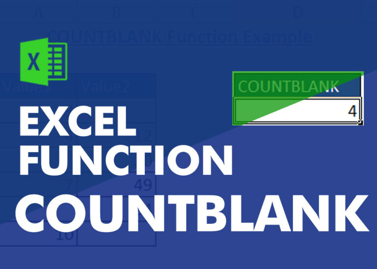
COUNTBLANK function is used to get the total count of Blank or Empty cell in range.
COUNTBLANK Function has one required argument i.e. range.
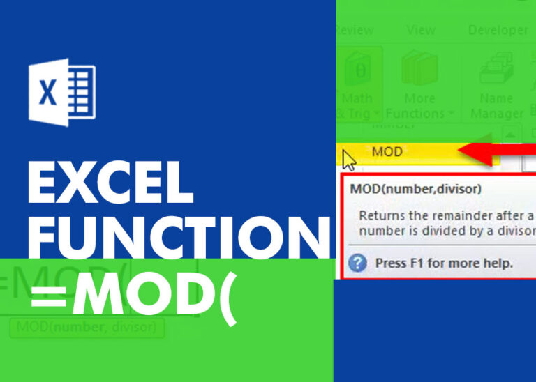
MOD function is used to get the remainder of number that is divided by divisor. MOD Function has two required arguments i.e. number and divisor.