EXCEL FUNCTION- LEFT
EXCEL FUNCTION LEFT
While working with Microsoft Excel, did you get a situation where you need to extract the Left side of characters from a string? I believe most of your answers are YES. In the said scenario “LEFT” function will help you to find the solution. We will be learning the Microsoft Excel “LEFT” in detail, so stay with us and continue reading…
LEFT function is used for extracting the “Left Most” characters from the available string. The output of the function returns the extracted characters in new cell.
Function should give output in “General” format, however if output is not as per the desired format then we need to change the cell format to “GENERAL”.
LEFT Function has two arguments i.e. text and num_chars where we need to give the cell references and parameters (i.e. count of characters required from left side in number format), we can give the parameters as per the requirement by following the “ , “ (i.e. Comma) as separator.
If parameters are not separated by “ , “ (i.e. Comma) or quotation mark is/are missing or any other function error then it will give output as “#VALUE!” (Error). So always ensure that function parameters are used to get the appropriate results/output.
Syntax:
=LEFT(text,num_chars)
Syntax Description:
text argument, is used to give the cell reference from which characters should be extracted
num_chars argument, is used to give the numeric value of total count of characters you want to extract from left side of a string
Advantages Of LEFT Functions
LEFT function is very advantageous in many ways. It helps for the document where extracting of characters from an available string is required. Extracting characters from an available string manually (one by one) to a report is very difficult and LEFT Function helps to apply the function in large database at once and makes the work easy, saves time and increases efficiency.
Example
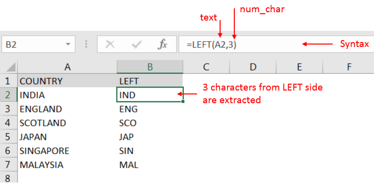
Suppose we have a column with Country names and there is requirement of extraction of first Left three character. We will be following LEFT function as follows:
“text argument”: “A2” is the cell reference from which characters should be extract
“num_char argument”: “3” is the total number of count of characters required from left side

Explanation: We can see in cell “A2” has string as “INDIA” and left function extracted total 3 characters from a sting and “IND” is returned as output in cell “B2”
Things to Remember:
– Spaces available in a string is counted as characters
– Currency symbols (Number Formatting) are not counted as characters and will be ignored by the function
– If “num_chars argument” field is blank, it will be counted as 1 (by default) and 1st character of the string will return as output
– “num_chars argument” should not be a negative value otherwise function output will return to “#VALUE!” (Error)
– If value in “num_chars argument” is greater than the total count of characters in a string, then function’s output will return the complete string.


