=MAX(number1,[number2],...)
number1 argument is required argument where we can give range or value
[number2] argument is optional argument where we can give another range or value
To create a MAX formula in simple way, you have to type numbers directly in the list of arguments, like this:
=MAX(1, 2, 3)
In practice, it’s quite a rare case when numbers are “hardcoded”. For the most part, you will deal with ranges and cells.
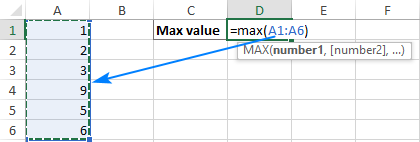
The fastest way to build a Max formula that finds the highest value in a range is this:

Decide where you want the maximum value to appear on your spreadsheet. This might be at the bottom of your data set, to the right or in any open cell. Click into the cell to select it.
Navigate to the “Home” tab on the ribbon. On the far right, you might see the sum symbol, which looks like a sigma. If you click the arrow to the right of the icon, it prompts a drop-down menu to open. Select “Max”.
The max function formula typically appears in the cell. You can then tell Excel which cell, array of cells or number to evaluate. You can do this by selecting a cell or range of cells or by manually typing in the arguments. You can then press “Enter”, prompting Excel to return the highest value.
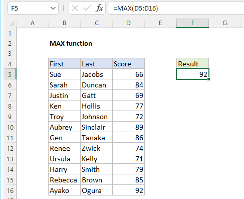
The MAX function returns the largest numeric value in the data provided. The MAX function can be used to return the largest value from any type of numeric data. For example, MAX can return the slowest time in a race, the latest date, the largest percentage, the highest temperature, or the top sales number.
The MAX function takes multiple arguments in the form number1, number2, number3, etc. up to 255 total. Arguments can be a hardcoded constant, a cell reference, or a range, in any combination. MAX ignores empty cells, text values, and the logical values TRUE and FALSE.
The MAX function returns the largest numeric value in supplied data:
=MAX(12,17,25,11,23) // returns 25
MAX ignores logical values and numbers entered as text, unless they are provided as arguments:
– Function will only consider numeric values while evaluating largest value
– Multiple ranges can be applied in function by separating them with comma (,)
– Text/ Spaces will be ignored by the function
– If No values in range or list of values (i.e. number argument) then output will return as 0 (zero)

Hope you learnt this Function,
Don’t forget to leave your valuable comments!
If you liked this article and want to learn more similar tricks, please Subscribe to us or follow us on Social Media by clicking the below buttons

Excel Function- WORKDAY.INTL WORKDAY.INTL function is an advanced version of WORKDAY function with additional advantage of “Custom weekend options” For Example, with WORKDAY function weekends are treated as “Saturday and Sundays” however if you need…

This guide shows three easy ways to make a histogram in Excel: using the built-in Histogram tool, formulas, or a PivotTable. Even though making charts is usually simple, histograms can be tricky. But in newer versions of Excel, it’s easy to create one in just a few steps. Let’s explore each method in detail.

How to count words in Excel using the LEN function along with other Excel functions. It also gives formulas for counting words or text, whether case-sensitive or not, in a cell or range.

COLUMN function is used to get the column reference number of the excel worksheet. COLUMN Function has only one argument.

COLUMNS function is used to get the total count of columns in an array or in cells range for excel worksheet.

COUNTA function is used to get the total count of Any-value or Non-Blanks in range. COUNTA Function has one required and optional argument: value1, value2