RANK function performs the Ranking in a range or list of numbers. Function returns the rank position and can assigned as Highest or Lowest value as 1st rank as per order argument.
Syntax:
=RANK(number,ref,[order])
number argument is used to give number value for which ranking is required
ref argument is used to give range or list of values from which rank to measure
[order] is optional argument and Value 0 or 1 can be given as per below requirements:
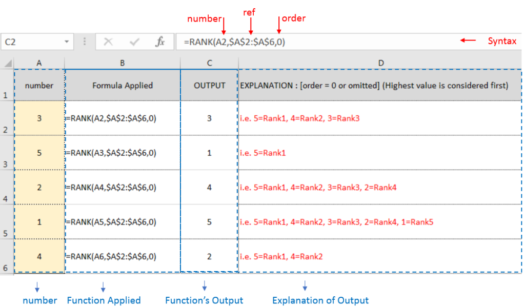
[order] = 0 or omitted: Highest value will be Ranked as 1st position (example: Value 5=Rank1, 4=Rank2, 3=Rank3, 2=Rank4, 1=Rank5 and so on)
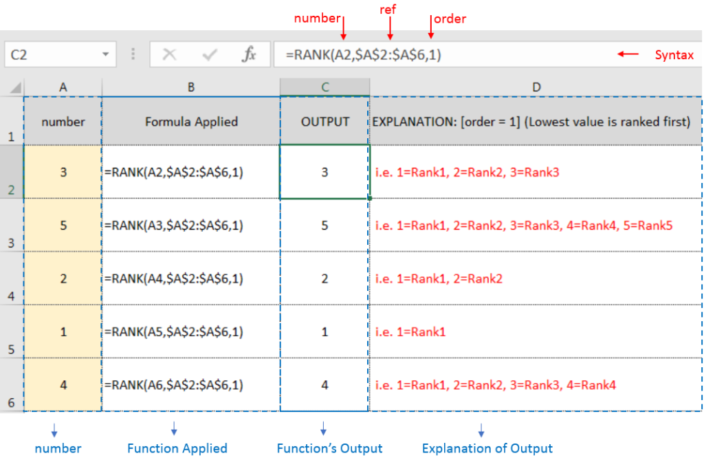
[order] = 1: Lowest value will be Ranked as 1st position (example: Value 1=Rank1, 2=Rank2, 3=Rank3, 4=Rank4, 5=Rank5 and so on)
Example 2: RANK function with [order = 1] (Lowest value is ranked first)
Example 3: RANK function with [order = 1] (Lowest value is ranked first) with Repeat values
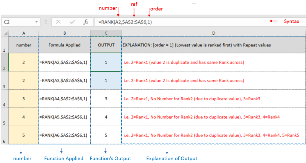
If list of values or ref argument has duplicate values, ranking for those values will be same across
Hope you learnt this Function,
Don’t forget to leave your valuable comments!
If you liked this article and want to learn more similar tricks, please Subscribe us or follow us on Social Media by clicking below buttons:

Understand how to find median in Excel with simple steps. Understanding the middle value in a set of numbers, known as the median, is important in the data industry. Professionals often use Microsoft Excel to calculate this. Excel’s MEDIAN function helps quickly find this value from long lists of numbers. This saves time and allows for further calculations using the median value. In this article, we explain what the MEDIAN function in Excel does, why it’s useful, and two methods to find the median in your data.
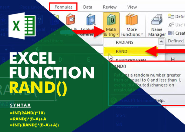
Generate Random Numbers in Excel Using RAND We have got many instances where we needed to generate a random database or values. Rand function is very useful for the users who creates random database for…
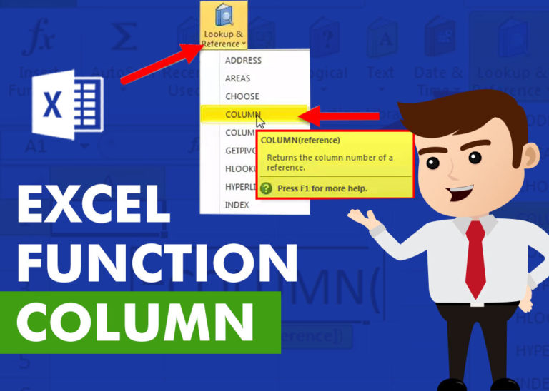
COLUMN function is used to get the column reference number of the excel worksheet. COLUMN Function has only one argument.

In an “IF function” there will be two output i.e. TRUE or FALSE since either the statement will be “TRUE” or “FALSE”. If the statement is matching or correct, then output will be “TRUE” or if the statement is not matching or not correct then the output will be “FALSE
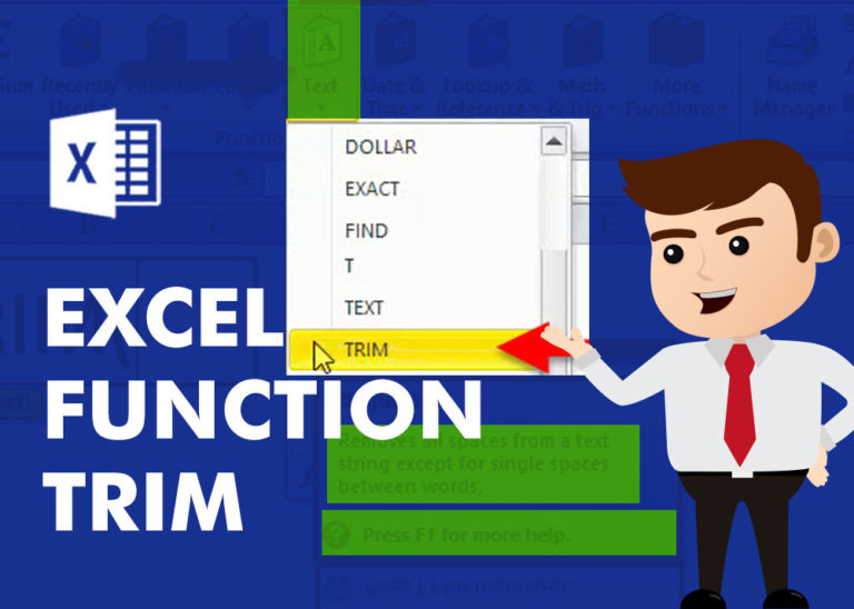
TRIM function is used to remove the additional spaces (i.e. spaces before/after/between the words) except for single space between words.

Watch: How to use COUNTIF & COUNTIFS Function in Excel? What is COUNTIF Function? In Excel, “COUNTIF” counts the number of cells within a range that meet a single specified criteria. Click here to Read…