=TEXT(value,format_text)
value argument [Required] is used to give the text or cell reference for which formatting is to be changed
format_text [Required], is used to give the formatting code as per the requirement
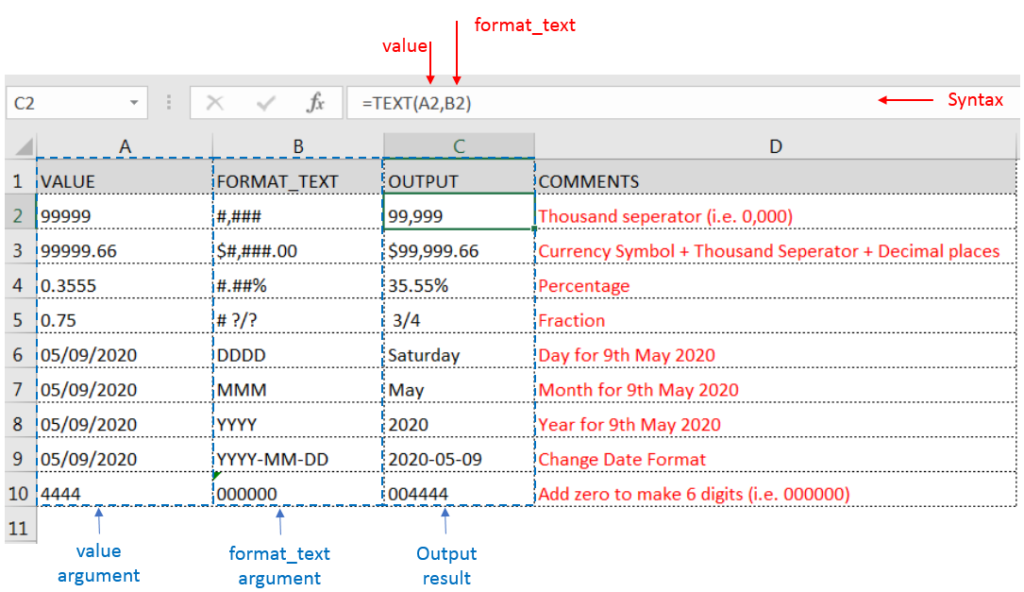
Here we have some examples, where “Column A” has various values, “Column B” represents format_text and “Column C” shows the output of the function.
We will be using TEXT function as follows:

– Format of cell can also be changed by following CTRL+1 (or MAC Command button +1) and select the desired format/appearance
– If cell reference is not correctly provided in the function, then it will give output as an error
– Function should give output in “General” format, however if output is not as per the desired format then we need to change the cell format to “GENERAL”
Hope you learnt this Function,
Don’t forget to leave your valuable comments!
If you liked this article and want to learn more similar tricks, please Subscribe us or follow us on Social Media by clicking below buttons:

SUBSTITUTE function is used to substitute the existing old text to new text.

SUMIF function is used to get the “total sum” for number of times the criteria across range is met. SUMIF Function has two required arguments.

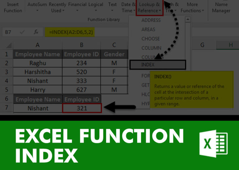
INDEX function is used to get the value from a cell range or table, function returns the value from a table where row and column intersect with each other.

FIND function is used to find the position of text, or character in an available string.

This guide shows how to use the nested IF function in Excel to check several conditions. You will also learn about other functions that can be to use than a nested formula.
When you want to make decisions in Excel, you often use an IF formula. It checks if something is true, then gives one result if it is and another result if it isn’t. If you need to check more than one thing, you can put many IFs inside each other.
Although using multiple IFs is common, it’s not the only way to check several conditions in Excel. This guide will introduce you to some easier and useful alternatives.

This tutorial shows you three easy ways to add hyperlinks in Excel. You will learn how to insert, change, and remove hyperlinks in your worksheets. It also explains how to fix links that don’t work.
Hyperlinks are often used on the internet to move between websites. In Excel, you can create links like that too. You can make a link to another cell, a different sheet, or even another workbook. You can also link to open a new Excel file or start an email message. This guide will show you how to do all of this in Excel 2016, 2013, 2010, and older versions.