Microsoft Excel “TODAY” function is used to get the current Date. It is very useful function and can be used in many ways. “TODAY Function” does not have any argument that makes this easy to apply and implement.
Date derived from TODAY function changes each time worksheet is refreshed/ edited/open/changed. So, ensure to Paste special values the formula output so that database is not changed. We will also discuss in below that how we can Paste special values.
“TODAY” function is very advantageous in many ways. It helps for the document where current Date details are required in more often. Applying current Date manually (one by one) to document is very difficult and “TODAY Function” helps to apply the function in large database at once and makes the work easy, saves time and increases efficiency.
“TODAY Function” is very useful and can be used in many situations. Like it can be used as follows:
– Document where Date stamps are required more often.
– Preparing time and motion study and day wise summary for employees
– Employees utilization or productivity, attendance tracker
– Or any other database where there is requirement of current Date stamps, “TODAY Function” can be used
=TODAY()
There are no arguments for “TODAY” function. Just apply the function and click “Enter”. It will show the current Date.
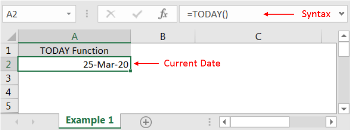
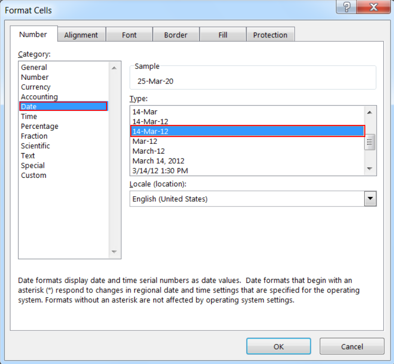
If output of the function is not as per the above (i.e. DATE), then we need to change the cell format. Follow below steps to change the format of the cell:
Step 1: Select the Cell or Data Range
Step 2: Press Ctrl + 1 to open “Format Cells” option
Step 3: Select the option as per below i.e. Date -> 14-Mar-12
Step 4: Click to “OK”
This will change the format of the cell to desired format. We can change ANY of the Date or Time format as given in “Format Cell” option.
Values derived from TODAY function changes each time worksheet is refreshed/ edited/open/changed. So, ensure to Paste special values the formula output so that database is not changed.
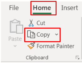
Below are the steps for paste special database to values:
– Select the data range -> Go to Menu Bar- > Click to Home-> Click to Copy
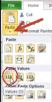
Then -> Go to Menu Bar- > Click to Home-> Click Paste Values
Hope you learnt this Function
Don’t forget to leave your valuable comments!
If you liked this article and want to learn more similar tricks, please Subscribe us.

INDIRECT function is used to convert the text/string into cell reference. Function provides output as the value of that cell reference.

LEN function is used for counting number of characters in available string. The output of the function returns the count in new cell.

MATCH function performs lookup for a value in a range and returns its position sequence number as output. It has two required and one optional arguments
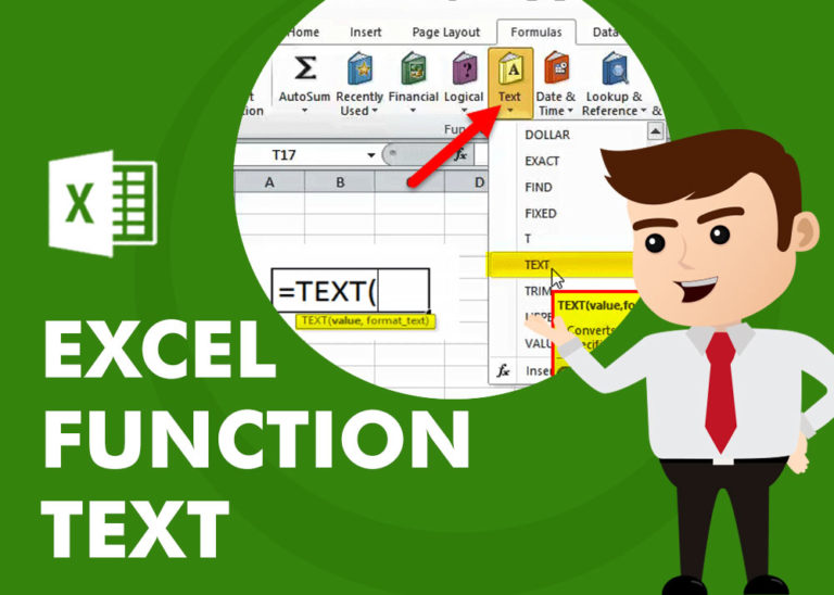
TEXT function is used to change the formatting or appearances of the text. There are various types of formatting available.

This tutorial explains how to use the IFERROR function in Excel to catch and handle errors. It shows you how to replace errors with a blank cell, a different value, or a custom message. You’ll also learn how to use IFERROR with functions like VLOOKUP and INDEX MATCH, and how it compares to other error-checking functions like IF ISERROR and IFNA

Watch: How to use VLOOKUP Function in Excel? What is VLOOKUP Function? The VLOOKUP function in Excel searches for a value in a table and returns a corresponding value from another column in the same row…